1. Introduction

This open-access textbook is, and will remain, freely available for everyone’s enjoyment (also in PDF; a paper copy can also be ordered). It is a non-profit project. Although available online, it is a whole course, and should be read from the beginning to the end. Refer to the Preface for general introductory remarks. Any bug/typo reports/fixes are appreciated. Make sure to check out Minimalist Data Wrangling with Python [28], too.

1.1. Hello, world!

Traditionally, every programming journey starts by printing a “Hello, world”-like greeting. Let’s then get it over with asap:

cat("My hovercraft is full of eels.\n")  # `\n` == newline
## My hovercraft is full of eels.

By calling (invoking) the cat function, we printed out a given character string that we enclosed in double-quote characters.

Documenting code is a good development practice. It is thus worth knowing that any text following a hash sign (that is not part of a string) is a comment. It is ignored by the interpreter.

# This is a comment.
# This is another comment.
cat("I cannot wait", "till lunchtime.\n")  # two arguments (another comment)
## I cannot wait till lunchtime.
cat("# I will not buy this record.\n# It is scratched.\n")
## # I will not buy this record.
## # It is scratched.

By convention, in this book, the textual outputs generated by R itself are always preceded by two hashes. This makes copy-pasting all code chunks easier in case we would like to experiment with them (which is always highly encouraged).

Whenever a call to a function is to be made, the round brackets are obligatory. All objects within the parentheses (they are separated by commas) constitute the input data to be consumed by the operation. Thus, the syntax is: a_function_to_call(argument1, argument2, etc.).

1.2. Setting up the development environment

1.2.1. Installing R

It is quite natural to pine for the ability to execute the foregoing code ourselves; to learn programming without getting our hands dirty is impossible.

The official precompiled binary distributions of R can be downloaded from https://cran.r-project.org/.

For serious programming work[1], we recommend, sooner rather than later, switching to[2] one of the UNIX-like operating systems. This includes the free, open-source (== good) variants of GNU/Linux, amongst others, or the proprietary (== not so good) m**OS. In such a case, we can employ our favourite package manager (e.g., apt, dnf, pacman, or Homebrew) to install R.

Other users (e.g., of Wi***ws) might consider installing Anaconda or Miniconda, especially if they would like to work with Jupyter (Section 1.2.5) or Python as well.

Below we review several ways in which we can write and execute R code. It is up to the benign readers to research, set up, and learn the development environment that suits their needs. As usual in real life, there is no single universal approach that always works best in all scenarios.

1.2.2. Interactive mode

Whenever we would like to compute something quickly, e.g., determine basic aggregates of a few numbers entered by hand or evaluate a mathematical expression like “2+2”, R’s read-eval-print loop (REPL) can give us instant gratification.

How to start the R console varies from system to system. For instance, the users of UNIX-like boxes can simply execute R from the terminal (shell, command line). Those on Wi***ws can activate RGui from the Start menu.

Important

When working interactively, the default[3] command prompt, “>”, means: I am awaiting orders. Moreover, “+” denotes: Please continue. In the latter case, we should either complete the unfinished expression or cancel the operation by pressing ESC or CTRL+C (depending on the operating system).

> cat("And now
+ for something
+ completely different
+
+
+ it is an unfinished expression...
+ awaiting another double quote character and then the closing bracket...
+
+ press ESC or CTRL+C to abort input
>

For readability, we never print out the command prompt characters in this book.

1.2.3. Batch mode: Working with R scripts (**)

The interactive mode of operation is unsuitable for more complicated tasks, though. The users of UNIX-like operating systems will be interested in another extreme, which involves writing standalone R scripts that can be executed line by line without any user intervention. To do so, in the terminal, we can invoke:

Rscript file.R

where file.R is the path to a source file; see Section 9.2.3 for more details

Exercise 1.1

(**) In your favourite text editor (e.g., Notepad++, Kate, vi, Emacs, RStudio, or VSCodium), create a file named test.R. Write a few calls to the cat function. Then, execute this script from the terminal through Rscript.

1.2.4. Weaving: Automatic report generation (**)

Reproducible data analysis[4] requires us to keep the results (text, tables, plots, auxiliary files) synchronised with the code and data that generate them.

utils::Sweave (the Sweave function from the utils package) and knitr [65] are two example template processors that evaluate R code chunks within documents written in LaTeX, HTML, or other markup languages. The chunks are replaced by the outputs they yield.

This book is a showcase of such an approach: all the results, including Figure 2.3 and the message about busy hovercrafts, were generated programmatically. Thanks to its being written in the highly universal Markdown language, it could be converted to a single PDF document as well as the whole website. This was facilitated by tools like pandoc and docutils.

Exercise 1.2

(**) Call install.packages("knitr") in R. Then, create a text file named test.Rmd with the following content:

# Hello, Markdown!

This is my first automatically generated report,
where I print messages and stuff.

```{r}
print("G'day!")
print(2+2)
plot((1:10)^2)
```

Thank you for your attention.

Assuming that the file is located in the current working directory (compare Section 7.3.2), call knitr::knit("test.Rmd") from the R console, or run in the terminal:

Rscript -e 'knitr::knit("test.Rmd")'

Inspect the generated Markdown file, test.md.

Furthermore, if you have the pandoc tool installed, to generate a standalone HTML file, execute in the terminal:

pandoc test.md --standalone -o test.html

Alternatively, see Section 7.3.2 for ways to call external programs from R.

1.2.5. Semi-interactive modes (Jupyter Notebooks, sending code to the associated R console, etc.)

The nature of the most frequent use cases of R encourages a semi-interactive workflow, where we quickly progress with prototyping by trial and error. In this mode, we compose a series of short code fragments inside a standalone R script. Each fragment implements a simple, well-defined task, such as loading data files, data cleansing, feature visualisation, computations of information aggregates, etc. Importantly, any code chunk can be sent to the associated R console and executed there. This way, we can inspect the result it generates. If we are not happy with the outcome, we can apply the necessary corrections.

There are quite a few integrated development environments that enable such a workflow, including JupyterLab, Emacs, RStudio, and VSCodium. Some of them require additional plugins for R.

Executing an individual code line or a whole text selection is usually done by pressing (configurable) keyboard shortcuts such as Ctrl+Enter or Shift+Enter.

Exercise 1.3

(*) JupyterLab is a development environment that runs in a web browser. It was programmed in Python, but supports many programming languages. Thanks to IRkernel, we can use it with R.

1. Install JupyterLab and IRkernel (for instance, if you use Anaconda, run conda install -c r r-essentials).

2. From the File menu, select Create a new R source file and save it as, e.g., test.R.

3. Click File and select Create a new console for the editor running the R kernel.

4. Input a few print “Hello, world”-like calls.

5. Press Shift+Enter (whilst working in the editor) to send different code fragments to the console and execute them. Inspect the results.

See Figure 1.1 for an illustration. Note that issuing options(jupyter.rich_display=FALSE) may be necessary to disable rich HTML outputs and make them look more like ones in this book.

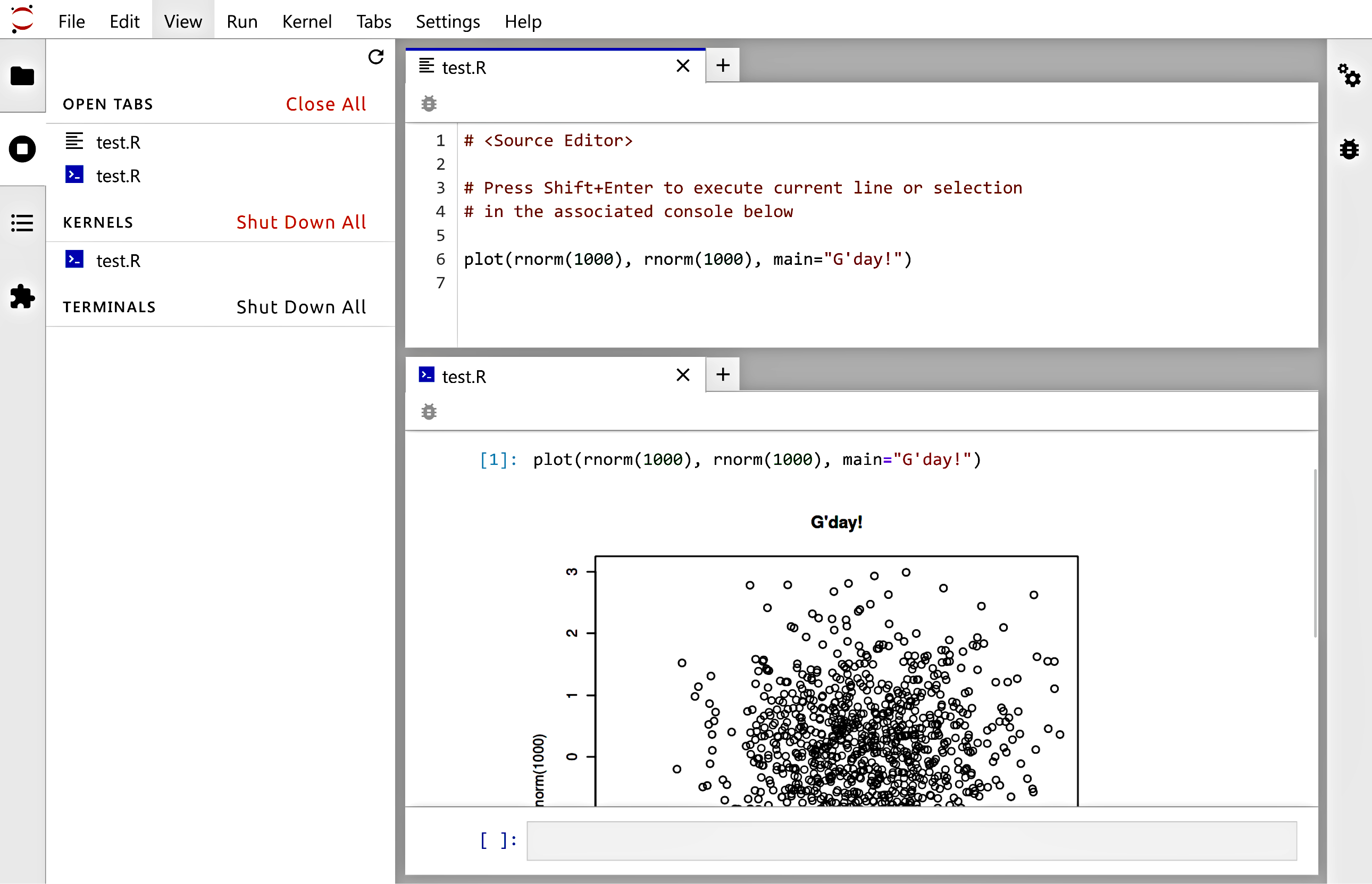
Figure 1.1 JupyterLab: A source file editor and the associated R console, where we can run arbitrary code fragments.

Example 1.4

(*) JupyterLab also handles dedicated Notebooks, where editable and executable code chunks and results they generate can be kept together in a single .ipynb (JSON) file; see Figure 1.2 for an illustration and Chapter 1 of [28] for a quick introduction (from the Python language kernel perspective).

This environment is convenient for live coding (e.g., for teachers) or performing exploratory data analyses. However, for more serious programming work, the code can get messy. Luckily, there is always an option to export a notebook to an executable, plain text R script.

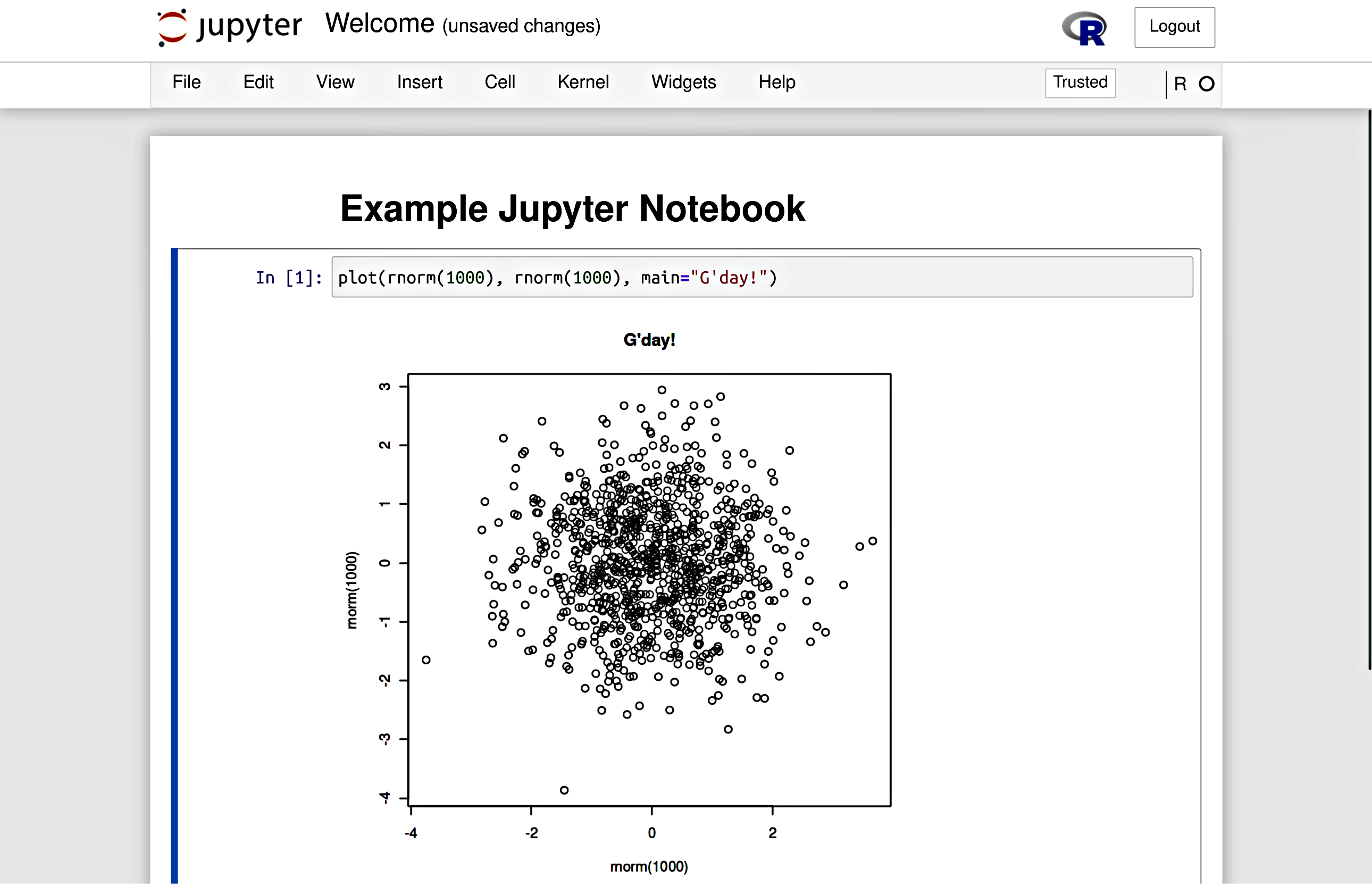
Figure 1.2 An example Jupyter Notebook, where we can keep code and results together.

1.3. Atomic vectors at a glance

After printing “Hello, world”, a typical programming course would normally proceed with the discussion on basic data types for storing individual numeric or logical values. Next, we would be introduced to arithmetic and relational operations on such scalars, followed by the definition of whole arrays or other collections of values, complemented by the methods to iterate over them, one element after another.

In R, no separate types representing individual values have been defined. Instead, what seems to be a single datum, is already a vector (sequence, array) of length one.

2.71828          # input a number; here: the same as print(2.71828)
## [1] 2.7183
length(2.71828)  # it is a vector with one element
## [1] 1

To create a vector of any length, we can call the c function, which combines given arguments into a single sequence:

c(1, 2, 3)  # three values combined
## [1] 1 2 3
length(c(1, 2, 3))  # indeed, it is a vector of length three
## [1] 3

In Chapter 2, Chapter 3, and Chapter 6, we will discuss the most prevalent types of atomic vectors: numeric, logical, and character ones, respectively.

c(0, 1, -3.14159, 12345.6)           # four numbers
## [1]     0.0000     1.0000    -3.1416 12345.6000
c(TRUE, FALSE)                       # two logical values
## [1]  TRUE FALSE
c("spam", "bacon", "spam")           # three character strings
## [1] "spam"  "bacon" "spam"

We call them atomic for they can only group together values of the same type. Lists, which we will discuss in Chapter 4, are, on the other hand, referred to as generic vectors. They can be used for storing items of mixed types: other lists as well.

Note

Not having separate scalar types greatly simplifies the programming of numerical computing tasks. Vectors are prevalent in our main areas of interest: statistics, simulations, data science, machine learning, and all other data-orientated computing. For example, columns and rows in tables (characteristics of clients, ratings of items given by users) or time series (stock market prices, readings from temperature sensors) are all best represented by means of such sequences.

The fact that vectors are the core part of the R language makes their use very natural, as opposed to the languages that require special add-ons for vector processing, e.g., numpy for Python [35]. By learning different ways to process them as a whole (instead of one element at a time), we will ensure that our ideas can quickly be turned into operational code. For instance, computing summary statistics such as, say, the mean absolute deviation of a sequence x, will be as effortless as writing mean(abs(x-mean(x))). Such code is not only easy to read and maintain, but it is also fast to run.

1.4. Getting help

Our aim is to become independent, advanced R programmers.

Independent, however, does not mean omniscient. The R help system is the authoritative source of knowledge about specific functions or more general topics. To open a help page, we call:

help("topic")  # equivalently: ?"topic"

Exercise 1.5

Sight (without going into detail) the manual on the length function by calling help("length"). Note that most help pages are structured as follows:

1. Header: package:base means that the function is a base one (see Section 7.3.1 for more details on the R package system);

2. Title;

3. Description: a short description of what the function does;

4. Usage: the list of formal arguments (parameters) to the function;

5. Arguments: the meaning of each formal argument explained;

6. Details: technical information;

7. Value: return value explained;

8. References: further reading;

9. See Also: links to other help pages;

10. Examples: R code that is worth inspecting.

We can also search within all the installed help pages by calling:

help.search("vague topic")  # equivalently: ??"vague topic"

This way, we will be able to find answers to our questions more reliably than when asking DuckDuckGo or G**gle, which commonly return many low-quality, irrelevant, or distracting results from splogs. We do not want to lose the sacred code writer’s flow! It is a matter of personal hygiene and good self discipline.

Important

All code chunks, including code comments and textual outputs, form an integral part of this book’s text. They should not be skipped by the reader. On the contrary, they must become objects of our intense reflection and thorough investigation.

For instance, whenever we introduce a function, it may be a clever idea to look it up in the help system. Moreover, playing with the presented code (running, modifying, experimenting, etc.) is also very beneficial. We should develop the habit of asking ourselves questions like “What would happen if…”, and then finding the answers on our own.

We are now ready to discuss the most significant operations on numeric vectors, which constitute the main theme of the next chapter. See you there.

1.5. Exercises

Exercise 1.6

What are the three most important types of atomic vectors?

Exercise 1.7

According to the classification of the R data types we introduced in the previous chapter, are atomic vectors basic or compound types?

---

[1]

For instance, when interoperability with other programming languages/environments is required or when we think about scheduling jobs on Linux-based computing/container clusters.

[2]

Or at least trying out – by installing a copy of GNU/Linux on a virtual machine (VM).

[3]

It can be changed; see help("options").

[4]

The idea dates back to Knuth’s literate programming concept; see [41].