5. Vector indexing

This open-access textbook is, and will remain, freely available for everyone’s enjoyment (also in PDF; a paper copy can also be ordered). It is a non-profit project. Although available online, it is a whole course, and should be read from the beginning to the end. Refer to the Preface for general introductory remarks. Any bug/typo reports/fixes are appreciated. Make sure to check out Minimalist Data Wrangling with Python [27] too.

We now know plenty of ways to process vectors in their entirety, but how to extract and replace their specific parts? We will be collectively referring to such activities as indexing. This is because they are often performed through the index operator, `[`.

5.1. head and tail

Let’s begin with something more lightweight, though. The head function fetches a few elements from the beginning of a vector.

x <- 1:10
head(x)  # head(x, 6)
## [1] 1 2 3 4 5 6
head(x, 3)   # get the first three
## [1] 1 2 3
head(x, -3)  # skip the last three
## [1] 1 2 3 4 5 6 7

Similarly, tail extracts a couple of items from the end of a sequence.

tail(x)  # tail(x, 6)
## [1]  5  6  7  8  9 10
tail(x, 3)   # get the last three
## [1]  8  9 10
tail(x, -3)  # skip the first three
## [1]  4  5  6  7  8  9 10

Both functions work on lists too[1]. They are useful for previewing the contents of really big objects. Also, they never complain about our trying to fetch too many elements:

head(x, 100)  # no more than the first 100 elements
##  [1]  1  2  3  4  5  6  7  8  9 10

5.2. Subsetting and extracting from vectors

Given a vector x, x[i] returns its subset comprised of elements indicated by the indexer i, which can be a single vector of:

• nonnegative integers (gives the positions of elements to retrieve),

• negative integers (gives the positions to omit),

• logical values (states which items should be fetched or skipped),

• character strings (locates the elements with specific names).

5.2.1. Nonnegative indexes

Consider example vectors:

(x <- seq(10, 100, 10))
##  [1]  10  20  30  40  50  60  70  80  90 100
(y <- list(1, 11:12, 21:23))
## [[1]]
## [1] 1
##
## [[2]]
## [1] 11 12
##
## [[3]]
## [1] 21 22 23

The first element in a vector is at index 1. Hence:

x[1]          # the first element
## [1] 10
x[length(x)]  # the last element
## [1] 100

Important

We might have wondered why “[1]” is displayed each time we print out an atomic vector on the console:

print((1:51)*10)
##  [1]  10  20  30  40  50  60  70  80  90 100 110 120 130 140 150 160 170
## [18] 180 190 200 210 220 230 240 250 260 270 280 290 300 310 320 330 340
## [35] 350 360 370 380 390 400 410 420 430 440 450 460 470 480 490 500 510

It is merely a visual hint indicating which vector element we output at the beginning in each line.

Vectorisation is a universal feature of R. It comes as no surprise that the indexer can also be of length greater than one.

x[c(1, length(x))]  # the first and the last
## [1]  10 100
x[1:3]  # the first three
## [1] 10 20 30

Take note of the boundary cases:

x[c(1, 2, 1, 0, 3, NA_real_, 1, 11)]  # repeated, 0, missing, out of bound
## [1] 10 20 10 30 NA 10 NA
x[c()]  # indexing by an empty vector
## numeric(0)

When applied on lists, the index operator always returns a list as well, even if we ask for a single element:

y[2]  # a list that includes the second element
## [[1]]
## [1] 11 12
y[c(1, 3)]  # not the same as x[1, 3] (a different story)
## [[1]]
## [1] 1
##
## [[2]]
## [1] 21 22 23

If we want to extract a component, i.e., to dig into what is inside a list at a specific location, we can refer to `[[`:

y[[2]]  # extract the second element
## [1] 11 12

This is exactly why R displays “[[1]]”, “[[2]]”, etc. when lists are printed.

On a side note, calling x[[i]] on an atomic vector, where i is a single value, has almost[2] the same effect as x[i]. However, `[[` generates an error if the subscript is out of bounds.

Important

Let’s reflect on the operators’ behaviour in the case of nonexistent items:

c(1, 2, 3)[4]
## [1] NA
list(1, 2, 3)[4]
## [[1]]
## NULL
c(1, 2, 3)[[4]]
## Error in c(1, 2, 3)[[4]]: subscript out of bounds
list(1, 2, 3)[[4]]
## Error in list(1, 2, 3)[[4]]: subscript out of bounds

Note

(*) `[[` also supports multiple indexers.

y[[c(1, 3)]]
## Error in y[[c(1, 3)]]: subscript out of bounds

Its meaning is different from y[c(1, 3)], though; we are about to extract a single value, remember? Here, indexing is applied recursively. Namely, the above is equivalent to y[[1]][[3]]. We got an error because y[[1]] is of a length smaller than three.

More examples:

y[[c(3, 1)]]  # y[[3]][[1]]
## [1] 21
list(list(7))[[c(1, 1)]]  # 7, not list(7)
## [1] 7

5.2.2. Negative indexes

The indexer can also be a vector of negative integers. This way, we can exclude the elements at given positions:

y[-1]  # all but the first
## [[1]]
## [1] 11 12
##
## [[2]]
## [1] 21 22 23
x[-(1:3)]  # all but the first three
## [1]  40  50  60  70  80  90 100
x[-c(1, 0, 2, 1, 1, 8:100)]  # 0, repeated, out of bound indexes
## [1] 30 40 50 60 70

Note

Negative and positive indexes cannot be mixed.

x[-1:3]  # recall that -1:3 == (-1):3
## Error in x[-1:3]: only 0's may be mixed with negative subscripts

Also, NA indexes cannot be mixed with negative ones.

5.2.3. Logical indexer

A vector can also be subsetted by means of a logical vector. If they both are of identical lengths, the consecutive elements in the latter indicate whether the corresponding elements of the indexed vector are supposed to be selected (TRUE) or omitted (FALSE).

#   1***  2      3      4      5***  6***  7      8***  9?   10***
x[c(TRUE, FALSE, FALSE, FALSE, TRUE, TRUE, FALSE, TRUE, NA,  TRUE)]
## [1]  10  50  60  80  NA 100

In other words, x[l], where l is a logical vector, returns all x[i] with i such that l[i] is TRUE. We thus extracted the elements at indexes 1, 5, 6, 8, and 10.

Important

Be careful: if the element selector is NA, we will get a missing value (for atomic vectors) or NULL (for lists).

c("one", "two", "three")[c(NA, TRUE, FALSE)]
## [1] NA    "two"
list("one", "two", "three")[c(NA, TRUE, FALSE)]
## [[1]]
## NULL
##
## [[2]]
## [1] "two"

This, lamentably, comes with no warning, which might be problematic when indexers are generated programmatically. As a remedy, we sometimes pass the logical indexer to the which function first. It returns the indexes of the elements equal to TRUE, ignoring the missing ones.

which(c(NA, TRUE, FALSE, TRUE, FALSE, NA, TRUE))
## [1] 2 4 7
c("one", "two", "three")[which(c(NA, TRUE, FALSE))]
## [1] "two"

Recall that in Chapter 3, we discussed ample vectorised operations that generate logical vectors. Anything that yields a logical vector of the same length as x can be passed as an indexer.

x > 60  # yes, it is a perfect indexer candidate
##  [1] FALSE FALSE FALSE FALSE FALSE FALSE  TRUE  TRUE  TRUE  TRUE
x[x > 60]  # select elements in `x` that are greater than 60
## [1]  70  80  90 100
x[x < 30 | 70 < x]  # elements not between 30 and 70
## [1]  10  20  80  90 100
x[x < mean(x)]  # elements smaller than the mean
## [1] 10 20 30 40 50
x[x^2 > 7777 | log10(x) <= 1.6]  # indexing via a transformed version of `x`
## [1]  10  20  30  90 100
(z <- round(runif(length(x)), 2))  # ten pseudorandom numbers
##  [1] 0.29 0.79 0.41 0.88 0.94 0.05 0.53 0.89 0.55 0.46
x[z <= 0.5]  # indexing based on `z`, not `x`: no problem
## [1]  10  30  60 100

The indexer is always evaluated first and then passed to the subsetting operation. The index operator does not care how an indexer is generated.

Furthermore, the recycling rule is applied when necessary:

x[c(FALSE, TRUE)]  # every second element
## [1]  20  40  60  80 100
y[c(TRUE, FALSE)]  # interestingly, there is no warning here
## [[1]]
## [1] 1
##
## [[2]]
## [1] 21 22 23

Exercise 5.1

Consider a simple database about six people, their favourite dishes, and birth years.

name <- c("Graham", "John", "Terry", "Eric",  "Michael", "Terry")
food <- c("bacon",  "spam", "spam",  "eggs",  "spam",    "beans")
year <- c( 1941,     1939,   1942,    1943,    1943,      1940  )

The consecutive elements in different vectors correspond to each other, e.g., Graham was born in 1941, and his go-to food was bacon.

• List the names of people born in 1941 or 1942.

• List the names of those who like spam.

• List the names of those who like spam and were born after 1940.

• Compute the average birth year of the lovers of spam.

• Give the average age, in 1969, of those who didn’t find spam utmostly delicious.

The answers must be provided programmatically, i.e., do not just write "Eric" and "Graham". Make the code generic enough so that it works in the case of any other database of this kind, no matter its size.

Exercise 5.2

Remove missing values from a given vector without referring to na.omit.

5.2.4. Character indexer

Let’s consider a vector equipped with the names attribute:

x <- structure(x, names=letters[1:10])  # add names
print(x)
##   a   b   c   d   e   f   g   h   i   j
##  10  20  30  40  50  60  70  80  90 100

These labels can be referred to when extracting the elements. To do this, we use an indexer that is a character vector:

x[c("a", "f", "a", "g", "z")]
##    a    f    a    g <NA>
##   10   60   10   70   NA

Important

We have said that special object attributes add extra functionality on top of the existing ones. Therefore, indexing by means of positive, negative, and logical vectors is still available:

x[1:3]
##  a  b  c
## 10 20 30
x[-(1:5)]
##   f   g   h   i   j
##  60  70  80  90 100
x[x > 70]
##   h   i   j
##  80  90 100

Lists can also be subsetted this way.

(y <- structure(y, names=c("first", "second", "third")))
## $first
## [1] 1
##
## $second
## [1] 11 12
##
## $third
## [1] 21 22 23
y[c("first", "second")]
## $first
## [1] 1
##
## $second
## [1] 11 12
y["third"]    # result is a list
## $third
## [1] 21 22 23
y[["third"]]  # result is the specific element unwrapped
## [1] 21 22 23

Important

Labels do not have to be unique. When we have repeated names, the first matching element is extracted:

structure(c(1, 2, 3), names=c("a", "b", "a"))["a"]
## a
## 1

There is no direct way to select all but given names, just like with negative integer indexers. For a workaround, see Section 5.4.1.

Exercise 5.3

Rewrite the solution to Exercise 5.1 assuming that we now have three features wrapped inside a list.

(people <- list(
    Name=c("Graham", "John", "Terry", "Eric",  "Michael", "Terry", "Steve"),
    Food=c("bacon",  "spam", "spam",  "eggs",  "spam",    "beans", "spam"),
    Year=c( 1941,     1939,   1942,    1943,    1943,      1940,   NA_real_)
))
## $Name
## [1] "Graham"  "John"    "Terry"   "Eric"    "Michael" "Terry"   "Steve"
##
## $Food
## [1] "bacon" "spam"  "spam"  "eggs"  "spam"  "beans" "spam"
##
## $Year
## [1] 1941 1939 1942 1943 1943 1940   NA

Do not refer to name, food, and year directly. Instead, use the full people[["Name"]] etc. accessors. There is no need to pout: it is just a tiny bit of extra work. Also, notice that Steve has joined the group; hello, Steve.

5.3. Replacing elements

5.3.1. Modifying atomic vectors

There are also replacement versions of the aforementioned indexing schemes. They allow us to substitute some new content for the old one.

(x <- 1:12)
##  [1]  1  2  3  4  5  6  7  8  9 10 11 12
x[length(x)] <- 42  # modify the last element
print(x)
##  [1]  1  2  3  4  5  6  7  8  9 10 11 42

The principles of vectorisation, recycling rule, and implicit coercion are all in place:

x[c(TRUE, FALSE)] <- c("a", "b", "c")
print(x)
##  [1] "a"  "2"  "b"  "4"  "c"  "6"  "a"  "8"  "b"  "10" "c"  "42"

Long story long: first, to ensure that the new content can be poured into the old wineskin, R coerced the numeric vector to a character one. Then, every second element therein, a total of six items, was replaced by a recycled version of the replacement sequence of length three. Finally, the name x was rebound to such a brought-forth object and the previous one became forgotten.

Note

For more details on replacement functions in general, see Section 9.3.6. Such operations alter the state of the object they are called on (quite rare a behaviour in functional languages).

Exercise 5.4

Replace missing values in a given numeric vector with the arithmetic mean of its well-defined observations.

5.3.2. Modifying lists

List contents can be altered as well. For modifying individual elements, the safest option is to use the replacement version of the `[[` operator:

y <- list(a=1, b=1:2, c=1:3)
y[[1]] <- 100:110
y[["c"]] <- -y[["c"]]
print(y)
## $a
##  [1] 100 101 102 103 104 105 106 107 108 109 110
##
## $b
## [1] 1 2
##
## $c
## [1] -1 -2 -3

The replacement version of `[` modifies a whole sub-list:

y[1:3] <- list(1, c("a", "b", "c"), c(TRUE, FALSE))
print(y)
## $a
## [1] 1
##
## $b
## [1] "a" "b" "c"
##
## $c
## [1]  TRUE FALSE

Moreover:

y[1] <- list(1:10)  # replace one element with one object
y[-1] <- 10:11      # replace two elements with two singletons
print(y)
## $a
##  [1]  1  2  3  4  5  6  7  8  9 10
##
## $b
## [1] 10
##
## $c
## [1] 11

Note

Let i be a vector of positive indexes of elements to be modified. Overall, calling “y[i] <- z” behaves as if we wrote:

1. y[[ i[1] ]] <- z[[1]],

2. y[[ i[2] ]] <- z[[2]],

3. y[[ i[3] ]] <- z[[3]],

and so forth.

Furthermore, z (but not i) will be recycled when necessary. In other words, we retrieve z[[j %% length(z)]] for consecutive js from 1 to the length of i.

Exercise 5.5

Reflect on the results of the following expressions:

• y[1] <- c("a", "b", "c"),

• y[[1]] <- c("a", "b", "c"),

• y[[1]] <- list(c("a", "b", "c")),

• y[1:3] <- c("a", "b", "c"),

• y[1:3] <- list(c("a", "b", "c")),

• y[1:3] <- "a",

• y[1:3] <- list("a"),

• y[c(1, 2, 1)] <- c("a", "b", "c").

Important

Setting a list item to NULL removes it from the list completely.

y <- list(1, 2, 3, 4)
y[1] <- NULL       # removes the first element (i.e., 1)
y[[1]] <- NULL     # removes the first element (i.e., now 2)
y[1] <- list(NULL) # sets the first element (i.e., now 3) to NULL
print(y)
## [[1]]
## NULL
##
## [[2]]
## [1] 4

The same notation convention is used for dropping object attributes; see Section 9.3.6.

5.3.3. Inserting new elements

New elements can be pushed at the end of the vector easily[3].

(x <- 1:5)
## [1] 1 2 3 4 5
x[length(x)+1] <- 6  # insert at the end
print(x)
## [1] 1 2 3 4 5 6
x[10] <- 10  # insert at the end but add more items
print(x)
##  [1]  1  2  3  4  5  6 NA NA NA 10

The elements to be inserted can be named as well:

x["a"] <- 11  # still inserts at the end
x["z"] <- 12
x["c"] <- 13
x["z"] <- 14  # z is already there; replace
print(x)
##                                a  z  c
##  1  2  3  4  5  6 NA NA NA 10 11 14 13

Note that x was not equipped with the names attribute before. The unlabelled elements were assigned blank labels (empty strings).

Note

It is not possible to insert new elements at the beginning or in the middle of a sequence, at least not with the index operator. By writing “x[3:4] <- 1:5” we do not replace two elements in the middle with five other ones. However, we can always use the c function to slice parts of the vector and intertwine them with some new content:

x <- seq(10, 100, 10)
x <- c(x[1:2], 1:5, x[5:7])
print(x)
##  [1] 10 20  1  2  3  4  5 50 60 70

5.4. Functions related to indexing

Let’s review a few operations which pinpoint interesting elements in a vector (or functions based on these).

5.4.1. Matching elements in another vector

We know that the `==` operator acts in an elementwise manner. It compares each element in a vector on its left side to the corresponding element in a vector on the right side. Thus, missing values and the recycling rule aside, if “z <- (x == y)”, then z[i] is TRUE if and only if x[i] is equal to y[i].

The `%in%` operator[4] is vectorised differently. It checks whether each element on the left-hand side matches one of the elements on the right. Given “z <- (x %in% y)”, z[i] is TRUE whenever x[i] is equal to y[j] for some j.

c("spam", "bacon", "spam", "eggs", "spam") %in% c("eggs", "spam", "ham")
## [1]  TRUE FALSE  TRUE  TRUE  TRUE

Example 5.6

Here is how we can remove the elements of a vector that have been assigned specified labels.

(x <- structure(1:12, names=month.abb))  # example vector
## Jan Feb Mar Apr May Jun Jul Aug Sep Oct Nov Dec
##   1   2   3   4   5   6   7   8   9  10  11  12
x[!(names(x) %in% c("Jan", "May", "Sep", "Oct"))]  # get rid of some elements
## Feb Mar Apr Jun Jul Aug Nov Dec
##   2   3   4   6   7   8  11  12

More generally, match(x, y) gives us the index of the element in y that matches each x[i].

match(c("spam", "bacon", "spam", "eggs", "spam"), c("eggs", "spam", "ham"))
## [1]  2 NA  2  1  2
match(month.abb, c("Jan", "May", "Sep", "Oct"))  # is the month on the list?
##  [1]  1 NA NA NA  2 NA NA NA  3  4 NA NA
match(c("Jan", "May", "Sep", "Oct"), month.abb)  # which month is it?
## [1]  1  5  9 10

By default, a missing value denotes a no-match.

Exercise 5.7

Check out the documentation of `%in%` to see how this operator is reduced to a call to match. Also, verify that it treats missing values as well-defined ones.

If the elements in y are not unique, the smallest index j such that x[i] == y[j] is returned. Therefore, for example, match(TRUE, l) fetches the index of the first occurrence of a positive value in a logical vector l.

(x <- round(runif(10), 2))  # example vector
##  [1] 0.29 0.79 0.41 0.88 0.94 0.05 0.53 0.89 0.55 0.46
match(TRUE, x>0.8)  # index of the first value > 0.8 (from the left)
## [1] 4

5.4.2. Assigning numbers into intervals

findInterval can come in handy where the assigning of numeric values into real intervals is needed. Namely, z <- findInterval(x, y) for increasing y gives z[i] being the index j such that x[i] is between y[j] (by default, inclusive) and y[j+1] (by default, exclusive).

For example, a sequence of five knots \(\boldsymbol{y}=(-\infty, 0.25, 0.5, 0.75, \infty)\) splits the real line into four intervals:

\[ \begin{array}{cccc} [-\infty, 0.25) & [0.25, 0.5) & [0.5, 0.75) & [0.75, \infty) \\ \text{\scriptsize (1)} & \text{\scriptsize (2)} & \text{\scriptsize (3)} & \text{\scriptsize (4)} \\ \end{array} \]

Hence, for instance:

findInterval(c(0, 0.2, 0.25, 0.4, 0.66, 1), c(-Inf, 0.25, 0.5, 0.75, Inf))
## [1] 1 1 2 2 3 4

Exercise 5.8

Refer to the manual of findInterval to verify the function’s behaviour when we do not include \(\pm\infty\) as endpoints and how to make \(\infty\) classified as a member of the fourth interval.

Exercise 5.9

Using a call to findInterval, compose a statement that generates a logical vector whose \(i\)-th element indicates whether x[i] is in the interval \([0.25, 0.5]\). Was this easier to write than an expression involving `<=` and `>=`?

5.4.3. Splitting vectors into subgroups

split(x, z) can take the output of match or findInterval (and many other operations) and divide the elements in a vector x into subgroups corresponding to identical zs.

For instance, we can assign people into groups determined by their favourite dish:

name <- c("Graham", "John", "Terry", "Eric",  "Michael", "Terry")
food <- c("bacon",  "spam", "spam",  "eggs",  "spam",    "beans")
split(name, food)  # group names with respect to food
## $bacon
## [1] "Graham"
##
## $beans
## [1] "Terry"
##
## $eggs
## [1] "Eric"
##
## $spam
## [1] "John"    "Terry"   "Michael"

The result is a named list with labels determined by the unique elements in the second vector.

Here is another example, where we pigeonhole some numbers into the four previously mentioned intervals:

x <- c(0, 0.2, 0.25, 0.4, 0.66, 1)
split(x, findInterval(x, c(-Inf, 0.25, 0.5, 0.75, Inf)))
## $`1`
## [1] 0.0 0.2
##
## $`2`
## [1] 0.25 0.40
##
## $`3`
## [1] 0.66
##
## $`4`
## [1] 1

Items in the first argument that correspond to missing values in the grouping vector will be ignored. Also, unsurprisingly, the recycling rule is applied when necessary.

We can also split x into groups defined by a combination of levels of two or more variables z1, z2, etc., by calling split(x, list(z1, z2, ...)).

Example 5.10

The ToothGrowth dataset is a named list (more precisely, a data frame; see Chapter 12) that represents the results of an experimental study involving 60 guinea pigs. The experiment’s aim was to measure the effect of different vitamin C supplement types and doses on the growth of the rodents’ teeth lengths:

ToothGrowth <- as.list(ToothGrowth)  # it is a list, but with extra attribs
ToothGrowth[["supp"]] <- as.character(ToothGrowth[["supp"]])  # was: factor
print(ToothGrowth)
## $len
##  [1]  4.2 11.5  7.3  5.8  6.4 10.0 11.2 11.2  5.2  7.0 16.5 16.5 15.2 17.3
## [15] 22.5 17.3 13.6 14.5 18.8 15.5 23.6 18.5 33.9 25.5 26.4 32.5 26.7 21.5
## [29] 23.3 29.5 15.2 21.5 17.6  9.7 14.5 10.0  8.2  9.4 16.5  9.7 19.7 23.3
## [43] 23.6 26.4 20.0 25.2 25.8 21.2 14.5 27.3 25.5 26.4 22.4 24.5 24.8 30.9
## [57] 26.4 27.3 29.4 23.0
##
## $supp
##  [1] "VC" "VC" "VC" "VC" "VC" "VC" "VC" "VC" "VC" "VC" "VC" "VC" "VC" "VC"
## [15] "VC" "VC" "VC" "VC" "VC" "VC" "VC" "VC" "VC" "VC" "VC" "VC" "VC" "VC"
## [29] "VC" "VC" "OJ" "OJ" "OJ" "OJ" "OJ" "OJ" "OJ" "OJ" "OJ" "OJ" "OJ" "OJ"
## [43] "OJ" "OJ" "OJ" "OJ" "OJ" "OJ" "OJ" "OJ" "OJ" "OJ" "OJ" "OJ" "OJ" "OJ"
## [57] "OJ" "OJ" "OJ" "OJ"
##
## $dose
##  [1] 0.5 0.5 0.5 0.5 0.5 0.5 0.5 0.5 0.5 0.5 1.0 1.0 1.0 1.0 1.0 1.0 1.0
## [18] 1.0 1.0 1.0 2.0 2.0 2.0 2.0 2.0 2.0 2.0 2.0 2.0 2.0 0.5 0.5 0.5 0.5
## [35] 0.5 0.5 0.5 0.5 0.5 0.5 1.0 1.0 1.0 1.0 1.0 1.0 1.0 1.0 1.0 1.0 2.0
## [52] 2.0 2.0 2.0 2.0 2.0 2.0 2.0 2.0 2.0

We can split len with respect to the combinations of supp and dose (also called interactions) by calling:

split(ToothGrowth[["len"]], ToothGrowth[c("supp", "dose")], sep="_")
## $OJ_0.5
##  [1] 15.2 21.5 17.6  9.7 14.5 10.0  8.2  9.4 16.5  9.7
##
## $VC_0.5
##  [1]  4.2 11.5  7.3  5.8  6.4 10.0 11.2 11.2  5.2  7.0
##
## $OJ_1
##  [1] 19.7 23.3 23.6 26.4 20.0 25.2 25.8 21.2 14.5 27.3
##
## $VC_1
##  [1] 16.5 16.5 15.2 17.3 22.5 17.3 13.6 14.5 18.8 15.5
##
## $OJ_2
##  [1] 25.5 26.4 22.4 24.5 24.8 30.9 26.4 27.3 29.4 23.0
##
## $VC_2
##  [1] 23.6 18.5 33.9 25.5 26.4 32.5 26.7 21.5 23.3 29.5

Other synonyms are, of course, possible, e.g., split(ToothGrowth[[1]], ToothGrowth[-1]) and split(ToothGrowth[[1]], list(ToothGrowth[[2]], ToothGrowth[[3]])). We recommend meditating upon our conscious use of double vs single square brackets here.

Functions such as Map (Section 7.2) will soon enable us to compute any summary statistics within groups, e.g., the group averages like those obtained by executing “SELECT AVG(len) FROM ToothGrowth GROUP BY supp, dose” in SQL. As an appetiser, let’s pass a list of vectors to the boxplot function; see Figure 5.1.

boxplot(split(ToothGrowth[["len"]], ToothGrowth[c("supp", "dose")], sep="_"))

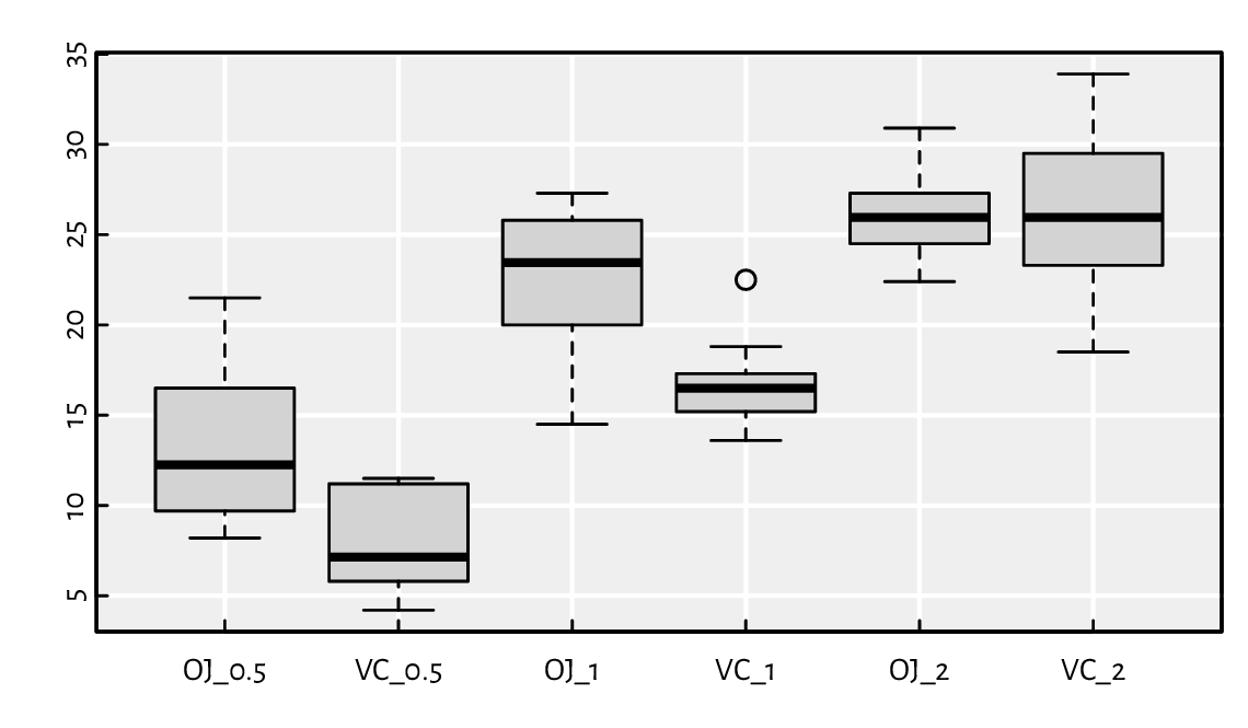
Figure 5.1 Box-and-whisker plots of len split by supp and dose in ToothGrowth.

Note

unsplit revokes the effects of split. Later, we will get used to calling unsplit(Map(some_transformation, split(x, z)), z) to modify the values in x independently in each group defined by z (e.g., standardise the variables within each class separately).

5.4.4. Ordering elements

The order function finds the ordering permutation of a given vector, i.e., a sequence of indexes that leads to a sorted version thereof.

x <- c(1024, 7, 42, 666, 0, 32787)
(o <- order(x))  # the ordering permutation of x
## [1] 5 2 3 4 1 6
x[o]  # ordered version of x
## [1]     0     7    42   666  1024 32787

Note that o[1] is the index of the smallest element in x, o[2] is the position of the second smallest, …, and o[length(o)] is the index of the greatest value. Hence, e.g., x[o[1]] is equivalent to min(x).

Another example:

x <- c("b", "a", "abs", "bass", "aaargh", "aargh", "aaaargh")
(o <- order(x))
## [1] 2 7 5 6 3 1 4
x[o]
## [1] "a"       "aaaargh" "aaargh"  "aargh"   "abs"     "b"       "bass"

Here, as x is a character vector, the ordering is lexicographical (like in a dictionary). This is exactly how `<=` on strings works.

Note

The ordering permutation that order returns is unique (that is why we call it the permutation), even for inputs containing duplicated elements. Owing to the use of a stable sorting algorithm, ties (repeated elements) will be listed in the order of occurrence.

order(c(10, 20, 40, 10, 10, 30, 20, 10, 10))
## [1] 1 4 5 8 9 2 7 6 3

We have, e.g., five 10s at positions 1, 4, 5, 8, and 9. These five indexes are guaranteed to be listed in this very order.

Ordering can also be performed in a nonincreasing manner:

x[order(x, decreasing=TRUE)]
## [1] "bass"    "b"       "abs"     "aargh"   "aaargh"  "aaaargh" "a"

Note

A call to sort(x) is equivalent to x[order(x)], but the former function can be faster in certain scenarios. For instance, one of its arguments can induce a partially sorted vector which can be helpful if we only seek a few order statistics (e.g., the seven smallest values). Speed is rarely a bottleneck in the case of sorting (when it is, we have a problem!). This is why we will not bother ourselves with such topics until the last part of this pleasant book. Currently, we aim at expanding our skill repertoire so that we can implement anything we can think of.

Exercise 5.11

is.unsorted(x) determines if the elements in x are… not sorted with respect to `<=`. Write an R expression that generates the same result by referring to the order function. Also, assuming that x is numeric, do the same by means of a call to diff.

order also accepts one or more arguments via the dot-dot-dot parameter, `...`. This way, we can sort a vector with respect to many criteria. If there are ties in the first variable, they will be resolved by the order of elements in the second variable. This is most useful for rearranging rows of a data frame, which we will exercise in Chapter 12.

x  <- c( 10,  20,  30,  40,  50,  60)
y1 <- c("a", "b", "a", "a", "b", "b")
y2 <- c("w", "w", "v", "u", "u", "v")
x[order(y1)]
## [1] 10 30 40 20 50 60
x[order(y2)]
## [1] 40 50 30 60 10 20
x[order(y1, y2)]
## [1] 40 30 10 50 60 20
x[order(y2, y1)]
## [1] 40 50 30 60 10 20

Note

(*) Calling order on a permutation (a vector that is an arbitrary arrangement of \(n\) consecutive natural numbers) determines its inverse.

x <- c(10, 30, 40, 20, 10, 10, 50, 30)
order(x)
## [1] 1 5 6 4 2 8 3 7
order(order(x))  # the inverse of the above permutation
## [1] 1 5 7 4 2 3 8 6
(x[order(x)])[order(order(x))]  # we get x again
## [1] 10 30 40 20 10 10 50 30

Note that order(order(x)) can be considered as a way to rank all the elements in x. For instance, the third value in x, 40, is assigned rank 7: it is the seventh smallest value in this vector. This breaks the ties on a first-come, first-served basis. But we can also write:

order(order(x, runif(length(x))))  # ranks with ties broken at random
## [1] 2 5 7 4 3 1 8 6

For different variations of these, see the rank function.

Exercise 5.12

Recall that sample(x) returns a pseudorandom permutation of elements of a given vector unless x is a single positive number. Write an expression that always produces a proper rearrangement, regardless of the size of x.

5.4.5. Identifying duplicates

Whether any element in a vector was already listed in the previous part of the sequence can be verified by calling:

x <- c(10, 20, 30, 20, 40, 50, 50, 50, 20, 20, 60)
duplicated(x)
##  [1] FALSE FALSE FALSE  TRUE FALSE FALSE  TRUE  TRUE  TRUE  TRUE FALSE

This function can be used to remove repeated observations; see also unique. This function returns a value that is not guaranteed to be sorted (unlike in some other languages/libraries).

Exercise 5.13

What can be the use case of a call to match(x, unique(x))?

Exercise 5.14

Given two named lists x and y, which we treat as key-value pairs, determine their set-theoretic union (with respect to the keys). For example:

x <- list(a=1, b=2)
y <- list(c=3, a=4)
z <- ...to.do...  # combine x and y
str(z)
## List of 3
##  $ a: num 4
##  $ b: num 2
##  $ c: num 3

5.4.6. Counting index occurrences

tabulate takes a vector of values from a set of small positive integers (e.g., indexes) and determines their number of occurrences:

x <- c(2, 4, 6, 2, 2, 2, 3, 6, 6, 3)
tabulate(x)
## [1] 0 4 2 1 0 3

In other words, there are 0 ones, 4 twos, …, and 3 sixes.

Exercise 5.15

Using a call to tabulate (amongst others), return a named vector with the number of occurrences of each unique element in a character vector. For example:

y <- c("a", "b", "a", "c", "a", "d", "e", "e", "g", "g", "c", "c", "g")
result <- ...to.do...
print(result)
## a b c d e g
## 3 1 3 1 2 3

5.5. Preserving and losing attributes

Attributes are conceived of as extra data. It is thus up to a function’s authors what they will decide to do with them. Generally, it is safe to assume that much thought has been put into the design of base R functions. Oftentimes, they behave fairly reasonably. This is why we are now going to spend some time now exploring their approaches to the handling of attributes.

Namely, for functions and operators that aim at transforming vectors passed as their inputs, the assumed strategy may be to:

• ignore the input attributes completely,

• equip the output object with the same set of attributes, or

• take care only of a few special attributes, such as names, if that makes sense.

Below we explore some common patterns; see also Section 1.3 of [68].

5.5.1. c

First, c drops[5] all attributes except names:

(x <- structure(1:4, names=c("a", "b", "c", "d"), attrib1="<3"))
## a b c d
## 1 2 3 4
## attr(,"attrib1")
## [1] "<3"
c(x)  # only `names` are preserved
## a b c d
## 1 2 3 4

We can therefore end up calling this function chiefly for this nice side effect. Also, recall that unname drops the labels.

unname(x)
## [1] 1 2 3 4
## attr(,"attrib1")
## [1] "<3"

5.5.2. as.something

as.vector, as.numeric, and similar drop all attributes in the case where the output is an atomic vector, but it might not necessarily do so in other cases (because they are S3 generics; see Chapter 10).

as.vector(x)  # drops all attributes if x is atomic
## [1] 1 2 3 4

5.5.3. Subsetting

Subsetting with `[` (except where the indexer is not given) drops all attributes but names (as well as dim and dimnames; see Chapter 11), which is adjusted accordingly:

x[1]    # subset of labels
## a
## 1
x[[1]]  # this always drops the labels (makes sense, right?)
## [1] 1

The replacement version of the index operator modifies the values in an existing vector whilst preserving all the attributes. In particular, skipping the indexer replaces all the elements:

y <- x
y[] <- c("u", "v")  # note that c("u", "v") has no attributes
print(y)
##   a   b   c   d
## "u" "v" "u" "v"
## attr(,"attrib1")
## [1] "<3"

5.5.4. Vectorised functions

Vectorised unary functions tend to copy all the attributes.

round(x)
## a b c d
## 1 2 3 4
## attr(,"attrib1")
## [1] "<3"

Binary operations are expected to get the attributes from the longer input. If they are of equal sizes, the first argument is preferred to the second.

y <- structure(c(1, 10), names=c("f", "g"), attrib1=":|", attrib2=":O")
y * x  # x is longer
##  a  b  c  d
##  1 20  3 40
## attr(,"attrib1")
## [1] "<3"
y[c("h", "i")] <- c(100, 1000)  # add two new elements at the end
y * x
##    f    g    h    i
##    1   20  300 4000
## attr(,"attrib1")
## [1] ":|"
## attr(,"attrib2")
## [1] ":O"
x * y
##    a    b    c    d
##    1   20  300 4000
## attr(,"attrib1")
## [1] "<3"
## attr(,"attrib2")
## [1] ":O"

Also, Section 9.3.6 mentions a way to copy all attributes from one object to another.

Important

Even in base R, the foregoing rules are not enforced strictly. We consider them inconsistencies that should be, for the time being, treated as features (with which we need to learn to live as they have not been fixed for years, but hope springs eternal).

As far as third-party extension packages are concerned, suffice it to say that a lot of R programmers do not know what attributes are whatsoever. It is always best to refer to the documentation, perform a few experiments, and/or manually ensure the preservation of the data we care about.

Exercise 5.16

Check what attributes are preserved by ifelse.

5.6. Exercises

Exercise 5.17

Answer the following questions (contemplate first, then use R to find the answer).

• What is the result of x[c()]? Is it the same as x[]?

• Is x[c(1, 1, 1)] equivalent to x[1]?

• Is x[1] equivalent to x["1"]?

• Is x[c(-1, -1, -1)] equivalent to x[-1]?

• What does x[c(0, 1, 2, NA)] do?

• What does x[0] return?

• What does x[1, 2, 3] do?

• What about x[c(0, -1, -2)] and x[c(-1, -2, NA)]?

• Why x[NA] is so significantly different from x[c(1, NA)]?

• What is x[c(FALSE, TRUE, 2)]?

• What will we obtain by calling x[x<min(x)]?

• What about x[length(x)+1]?

• Why x[min(y)] is most probably a mistake? What could it mean? How can it be fixed?

• Why cannot we mix indexes of different types and write x[c(1, "b", "c", 4)]? Or can we?

• Why would we call as.vector(na.omit(x)) instead of just na.omit(x)?

• What is the difference between sort and order?

• What is the type and the length of the object returned by a call to split(a, u)? What about split(a, c(u, v))?

• How to get rid of the seventh element from a list of ten elements?

• How to get rid of the seventh, eight, and ninth elements from a list with ten elements?

• How to get rid of the seventh element from an atomic vector of ten elements?

• If y is a list, by how many elements “y[c(length(y)+1, length(y)+1, length(y)+1)] <- list(1, 2, 3)” will extend it?

• What is the difference between x[x>0] and x[which(x>0)]?

Exercise 5.18

If x is an atomic vector of length n, x[5:n] obviously extracts everything from the fifth element to the end. Does it, though? Check what happens when x is of length less than five, including 0. List different ways to correct this expression so that it makes (some) sense in the case of shorter vectors.

Exercise 5.19

Similarly, x[length(x) + 1 - 5:1] is supposed to return the last five elements in x. Propose a few alternatives that are correct also for short xs.

Exercise 5.20

Given a numeric vector, fetch its five largest elements. Ensure the code works for vectors of length less than five.

Exercise 5.21

We can compute a trimmed mean of some x by setting the trim argument to the mean function. Compute a similar robust estimator of location – the \(p\)-winsorised mean, \(p\in[0, 0.5]\) defined as the arithmetic mean of all elements in x clipped to the \([Q_p, Q_{1-p}]\) interval, where \(Q_p\) is the vector’s \(p\)-quantile; see quantile. For example, if x is (8, 5, 2, 9, 7, 4, 6, 1, 3), we have \(Q_{0.25}=3\) and \(Q_{0.75}=7\) and hence the \(0.25\)-winsorised mean will be equal to the arithmetic mean of (7, 5, 3, 7, 7, 4, 6, 3, 3).

Exercise 5.22

Let x and y be two vectors of the same length, \(n\), and no ties. Implement the formula for the Spearman rank correlation coefficient:

\[ \varrho(\mathbf{x},\mathbf{y}) = 1-\frac{6 \sum_{i=1}^n d_i^2}{n (n^2-1)}, \]

where \(d_i=r_i-s_i\), \(i=1,\dots,n\), and \(r_i\) and \(s_i\) denote the rank of \(x_i\) and \(y_i\), respectively; see also cor.

Exercise 5.23

(*) Given two vectors x and y both of length \(n\), a call to approx(x, y, ...) can be used to interpolate linearly between the points \((x_1, y_1), (x_2, y_2), \dots, (x_n, y_n)\). We can use it to generate new \(y\)s for previously unobserved \(x\)s (somewhere “in-between” the data we already have). Moreover, spline(x, y, ...) can perform a cubic spline interpolation, which is smoother; see Figure 5.2.

x <- c(1, 3,  5, 7, 10)
y <- c(1, 15, 25, 6,  0)
x_new <- seq(1, 10, by=0.25)
y_new1 <- approx(x, y, xout=x_new)[["y"]]
y_new2 <- spline(x, y, xout=x_new)[["y"]]
plot(x, y, ylim=c(-10, 30))  # the points to interpolate between
lines(x_new, y_new1, col="black", lty="solid")  # linear interpolation
lines(x_new, y_new2, col="darkred", lty="dashed")  # cubic interpolation
legend("topright", legend=c("linear", "cubic"),
    lty=c("solid", "dashed"), col=c("black", "darkred"), bg="white")

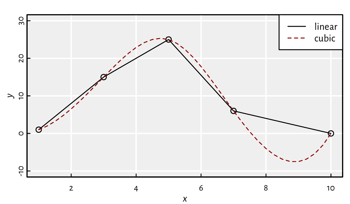
Figure 5.2 Piecewise linear and cubic spline interpolation.

Using a call to one of the above, impute missing data in euraud-20200101-20200630.csv, e.g., the blanks in (0.60, 0.62, NA, 0.64, NA, NA, 0.58) should be filled so as to obtain (0.60, 0.62, 0.63, 0.64, 0.62, 0.60, 0.58).

Exercise 5.24

Given some 1 ≤ from ≤ to ≤ n, use findInterval to generate a logical vector of length n with TRUE elements only at indexes between from and to, inclusive.

Exercise 5.25

Implement expressions that give rise to the same results as calls to which, which.min, which.max, and rev functions. What is the difference between x[x>y] and x[which(x>y)]? What about which.min(x) vs which(x == min(x))?

Exercise 5.26

Given two equal-length vectors x and y, fetch the value from the former that corresponds to the smallest value in the latter. Write three versions of such an expression, each dealing with potential ties in y differently. For example:

x <- c("a", "b", "c", "d", "e", "f")
y <- c(  3,   1,   2,   1,   1,   4)

It should choose the first ("b"), last ("e"), or random element from x fulfilling the above property ("b", "d", or "e" with equal probability). Make sure your code works for x being of the type character or numeric as well as an empty vector.

Exercise 5.27

Implement an expression that yields the same result as duplicated(x) for a numeric vector x, but using diff and order.

Exercise 5.28

Based on match and unique, implement your versions of union(x, y), intersect(x, y), setdiff(x, y), is.element(x, y), and setequal(x, y) for x and y being nonempty numeric vectors.

---

[1]

head and tail are actually S3 generics defined in the utils package. We are able to call them on matrices and data frames; see Chapter 10.

[2]

See also Section 5.5 for the discussion on the preservation of object attributes.

[3]

And often cheaply; see Section 8.3.5 for performance notes. Still, a warning can be generated on each size extension if the "check.bounds" flag is set; see help("options").

[4]

A fantastic name; see Section 9.3.5.

[5]

To be precise, we mean the default S3 method of c here; compare Section 10.2.4.