2. Numeric vectors

This open-access textbook is, and will remain, freely available for everyone’s enjoyment (also in PDF; a paper copy can also be ordered). It is a non-profit project. Although available online, it is a whole course, and should be read from the beginning to the end. Refer to the Preface for general introductory remarks. Any bug/typo reports/fixes are appreciated. Make sure to check out Minimalist Data Wrangling with Python [27] too.

In this chapter, we discuss the uttermost common operations on numeric vectors. They are so fundamental that we will also find them in other scientific computing environments, including Python with numpy or tensorflow, Julia, MATLAB, GNU Octave, or Scilab.

At first blush, the number of functions we are going to explore may seem quite large. Still, the reader is kindly asked to place some trust (a rare thing these days) in yours truly. It is because our selection is comprised only of the most representative and educational amongst the plethora of possible choices. More complex building blocks can often be reduced to a creative combination of the former or be easily found in a number of additional packages or libraries (e.g., GNU GSL [28]).

A solid understanding of base R programming is crucial for dealing with popular packages (such as data.table, dplyr, or caret). Most importantly, base R’s API is stable. Hence, the code we compose today will most likely work the same way in ten years. It is often not the case when we rely on external add-ons.

In the sequel, we will be advocating a minimalist, keep-it-simple approach to the art of programming data processing pipelines, one that is a healthy balance between “doing it all by ourselves”, “minimising the information overload”, “being lazy”, and “standing on the shoulders of giants”.

Note

The exercises that we suggest in the sequel are all self-contained, unless explicitly stated otherwise. The use of language constructs that are yet to be formally introduced (in particular, if, for, and while explained in Chapter 8) is not just unnecessary: it is discouraged. Moreover, we recommend against taking shortcuts by looking up partial solutions on the internet. Rather, to get the most out of this course, we should be seeking relevant information within the current and preceding chapters as well as the R help system.

2.1. Creating numeric vectors

2.1.1. Numeric constants

The simplest numeric vectors are those of length one:

-3.14
## [1] -3.14
1.23e-4
## [1] 0.000123

The latter is in what we call scientific notation, which is a convenient means of entering numbers of very large or small orders of magnitude. Here, “e” stands for “… times 10 to the power of…”. Therefore, 1.23e-4 is equal to \(1.23\times 10^{-4}=0.000123\). In other words, given \(1.23\), we move the decimal separator by four digits towards the left, adding zeroes if necessary.

In real life, some information items may be inherently or temporarily missing, unknown, or Not Available. As R is orientated towards data processing, it was equipped with a special indicator:

NA_real_  # numeric NA (missing value)
## [1] NA

It is similar to the Null marker in database query languages such as SQL. Note that NA_real_ is displayed simply as “NA”, chiefly for readability.

Moreover, Inf denotes infinity, \(\infty\), i.e., an element that is larger than the largest representable double-precision (64 bit) floating point value. Also, NaN stands for not-a-number, which is returned as the result of some illegal operations, e.g., \(0/0\) or \(\infty-\infty\).

Let’s provide a few ways to create numeric vectors with possibly more than one element.

2.1.2. Concatenating vectors with c

First, the c function can be used to combine (concatenate) many numeric vectors, each of any length. It results in a single object:

c(1, 2, 3)  # three vectors of length one –> one vector of length three
## [1] 1 2 3
c(1, c(2, NA_real_, 4), 5, c(6, c(7, Inf)))
## [1]   1   2  NA   4   5   6   7 Inf

Note

Running help("c"), we will see that its usage is like c(...). In the current context, this means that the c function takes an arbitrary number of arguments. In Section 9.4.6, we will study the dot-dot-dot (ellipsis) parameter in more detail.

2.1.3. Repeating entries with rep

Second, rep replicates the elements in a vector a given number of times.

rep(1, 5)
## [1] 1 1 1 1 1
rep(c(1, 2, 3), 4)
##  [1] 1 2 3 1 2 3 1 2 3 1 2 3

In the second case, the whole vector (1, 2, 3) has been recycled (tiled) four times. Interestingly, if the second argument is a vector of the same length as the first one, the behaviour will be different:

rep(c(1, 2, 3), c(2, 1, 4))
## [1] 1 1 2 3 3 3 3
rep(c(1, 2, 3), c(4, 4, 4))
##  [1] 1 1 1 1 2 2 2 2 3 3 3 3

Here, each element is repeated the corresponding number of times.

Calling help("rep"), we find that the function’s usage is like rep(x, ...). It is rather peculiar. However, reading further, we discover that the ellipsis (dot-dot-dot) may be fed with one of the following parameters:

• times,

• length.out[1],

• each.

So far, we have been playing with times, which is listed second in the parameter list (after x, the vector whose elements are to be repeated).

Important

It turns out that the undermentioned function calls are all equivalent:

rep(c(1, 2, 3), 4)   # positional matching of arguments: `x`, then `times`
rep(c(1, 2, 3), times=4)    # `times` is the second argument
rep(x=c(1, 2, 3), times=4)  # keyword arguments of the form name=value
rep(times=4, x=c(1, 2, 3))  # keyword arguments can be given in any order
rep(times=4, c(1, 2, 3))    # mixed positional and keyword arguments

We can also pass each or length.out, but their names must be mentioned explicitly:

rep(c(1, 2, 3), length.out=7)
## [1] 1 2 3 1 2 3 1
rep(c(1, 2, 3), each=3)
## [1] 1 1 1 2 2 2 3 3 3
rep(c(1, 2, 3), length.out=7, each=3)
## [1] 1 1 1 2 2 2 3

Note

Whether it was a good programming practice to actually implement a range of varied behaviours inside a single function is a matter of taste. On the one hand, in all of the preceding examples, we do repeat the input elements somehow, so remembering just one function name is really convenient. Nevertheless, a drastic change in the repetition pattern depending, e.g., on the length of the times argument can be bug-prone. Anyway, we have been warned[2].

Zero-length vectors are possible too:

rep(c(1, 2, 3), 0)
## numeric(0)

Even though their handling might be a little tricky, we will later see that they are indispensable in contexts like “create an empty data frame with a specific column structure”.

Also, note that R often allows for partial matching of named arguments, but its use is a bad programming practice; see Section 15.4.4 for more details.

rep(c(1, 2, 3), len=7)  # not recommended (see later)
## Warning in rep(c(1, 2, 3), len = 7): partial argument match of 'len' to
##     'length.out'
## [1] 1 2 3 1 2 3 1

We see the warning only because we have set options(warnPartialMatchArgs=TRUE) in our environment. It is not used by default.

2.1.4. Generating arithmetic progressions with seq and `:`

Third, we can call the seq function to create a sequence of equally-spaced numbers on a linear scale, i.e., an arithmetic progression.

seq(1, 15, 2)
## [1]  1  3  5  7  9 11 13 15

From the function’s help page, we discover that seq accepts the from, to, by, and length.out arguments, amongst others. Thus, the preceding call is equivalent to:

seq(from=1, to=15, by=2)
## [1]  1  3  5  7  9 11 13 15

Note that to actually means “up to”:

seq(from=1, to=16, by=2)
## [1]  1  3  5  7  9 11 13 15

We can also pass length.out instead of by. In such a case, the increments or decrements will be computed via the formula ((to - from)/(length.out - 1)). This default value is reported in the Usage section of help("seq").

seq(1, 0, length.out=5)
## [1] 1.00 0.75 0.50 0.25 0.00
seq(length.out=5)  # default `from` is 1
## [1] 1 2 3 4 5

Arithmetic progressions with steps equal to 1 or -1 can also be generated via the `:` operator.

1:10    # seq(1, 10) or seq(1, 10, 1)
##  [1]  1  2  3  4  5  6  7  8  9 10
-1:10   # seq(-1, 10) or seq(-1, 10, 1)
##  [1] -1  0  1  2  3  4  5  6  7  8  9 10
-1:-10  # seq(-1, -10) or seq(-1, -10, -1)
##  [1]  -1  -2  -3  -4  -5  -6  -7  -8  -9 -10

Let’s highlight the order of precedence of this operator: -1:10 means (-1):10, and not -(1:10); compare Section 2.4.3.

Exercise 2.1

Take a look at the manual page of seq_along and seq_len and determine whether we can do without them, having seq[3] at hand.

2.1.5. Generating pseudorandom numbers

We can also generate sequences drawn independently from a range of univariate probability distributions.

runif(7)  # uniform U(0, 1)
## [1] 0.287578 0.788305 0.408977 0.883017 0.940467 0.045556 0.528105
rnorm(7)  # normal N(0, 1)
## [1]  1.23950 -0.10897 -0.11724  0.18308  1.28055 -1.72727  1.69018

These correspond to seven pseudorandom deviates from the uniform distribution on the unit interval (i.e., \((0, 1)\)) and the standard normal distribution (i.e., with expectation 0 and standard deviation 1), respectively; compare Figure 2.3.

For more named distribution classes frequently occur in various real-world statistical modelling exercises, see Section 2.3.4.

Another worthwhile function picks items from a given vector, either with or without replacement:

sample(1:10, 20, replace=TRUE)  # 20 with replacement (allow repetitions)
##  [1]  3  3 10  2  6  5  4  6  9 10  5  3  9  9  9  3  8 10  7 10
sample(1:10, 5, replace=FALSE)  # 5 without replacement (do not repeat)
## [1] 9 3 4 6 1

The distribution of the sampled values does not need to be uniform; the prob argument may be fed with a vector of the corresponding probabilities. For example, here are 20 independent realisations of the random variable \(X\) such that \(\Pr(X=0)=0.9\) (the probability that we obtain 0 is equal to 90%) and \(\Pr(X=1)=0.1\):

sample(0:1, 20, replace=TRUE, prob=c(0.9, 0.1))
##  [1] 0 0 0 0 1 0 0 0 0 0 1 0 0 0 0 0 0 0 0 1

Note

If n is a single number (a numeric vector of length 1), then sample(n, ...) is equivalent to sample(1:n, ...). Similarly, seq(n) is a synonym for seq(1, n) or seq(1, length(n)), depending on the length of n. This is a dangerous behaviour that can occasionally backfire and lead to bugs (check what happens when n is, e.g., 0). Nonetheless, we have been warned. From now on, we are going to be extra careful (but are we really?). Read more at help("sample") and help("seq").

Let’s stress that the numbers we obtain are merely pseudorandom because they are generated algorithmically. R uses the Mersenne-Twister MT19937 method [46] by default; see help("RNG") and [21, 29, 42]. By setting the seed of the random number generator, i.e., resetting its state to a given one, we can obtain results that are reproducible.

set.seed(12345)  # seeds are specified with integers
sample(1:10, 5, replace=TRUE)  # a,b,c,d,e
## [1]  3 10  8 10  8
sample(1:10, 5, replace=TRUE)  # f,g,h,i,j
## [1]  2  6  6  7 10

Setting the seed to the one used previously gives:

set.seed(12345)
sample(1:10, 5, replace=TRUE)  # a,b,c,d,e
## [1]  3 10  8 10  8

We did not(?) expect that! And now for something completely different:

set.seed(12345)
sample(1:10, 10, replace=TRUE)  # a,b,c,d,e,f,g,h,i,j
##  [1]  3 10  8 10  8  2  6  6  7 10

Reproducibility is a crucial feature of each truly scientific experiment. The same initial condition (here: the same seed) leads to exactly the same outcomes.

Note

Some claim that the only unsuspicious seed is 42 but in matters of taste, there can be no disputes. Everyone can use their favourite picks: yours truly savours 123, 1234, and 12345 as well.

When performing many runs of Monte Carlo experiments, it may also be a clever idea to call set.seed(i) in the \(i\)-th iteration of a simulation we are trying to program.

We should ensure that our seed settings are applied consistently across all our scripts. Otherwise, we might be accused of tampering with evidence. For instance, here is the ultimate proof that we are very lucky today:

set.seed(1679619)  # totally unsuspicious, right?
sample(0:1, 20, replace=TRUE)  # so random
##  [1] 1 1 1 1 1 1 1 1 1 1 1 1 1 1 1 1 1 1 1 1

This is exactly why reproducible scripts and auxiliary data should be published alongside all research reports or papers. Only open, transparent science can be fully trustworthy.

If set.seed is not called explicitly, and the random state is not restored from the previously saved R session (see Chapter 16), then the random generator is initialised based on the current wall time and the identifier of the running R instance (PID). This may justify the impression that the numbers we generate appear surprising.

To understand the “pseudo” part of the said randomness better, in Section 8.3, we will build a very simple random generator ourselves.

2.1.6. Reading data with scan

An example text file named euraud-20200101-20200630.csv gives the EUR to AUD exchange rates (how many Australian Dollars can we buy for 1 Euro) from 1 January to 30 June 2020 (remember COVID-19?). Let’s preview the first couple of lines:

# EUR/AUD Exchange Rates
# Source: Statistical Data Warehouse of the European Central Bank System
# https://www.ecb.europa.eu/stats/policy_and_exchange_rates/
# (provided free of charge)
NA
1.6006
1.6031
NA

The four header lines that begin with “#” merely serve as comments for us humans. They should be ignored by the interpreter. The first “real” value, NA, corresponds to 1 January (Wednesday, New Year’s Day; Forex markets were closed, hence a missing observation).

We can invoke the scan function to read all the inputs and convert them to a single numeric vector:

scan(paste0("https://github.com/gagolews/teaching-data/raw/",
    "master/marek/euraud-20200101-20200630.csv"), comment.char="#")
##  [1]     NA 1.6006 1.6031     NA     NA 1.6119 1.6251 1.6195 1.6193 1.6132
## [11]     NA     NA 1.6117 1.6110 1.6188 1.6115 1.6122     NA     NA 1.6154
## [21] 1.6177 1.6184 1.6149 1.6127     NA     NA 1.6291 1.6290 1.6299 1.6412
## [31] 1.6494     NA     NA 1.6521 1.6439 1.6299 1.6282 1.6417     NA     NA
## [41] 1.6373 1.6260 1.6175 1.6138 1.6151     NA     NA 1.6129 1.6195 1.6142
## [51] 1.6294 1.6363     NA     NA 1.6384 1.6442 1.6565 1.6672 1.6875     NA
## [61]     NA 1.6998 1.6911 1.6794 1.6917 1.7103     NA     NA 1.7330 1.7377
## [71] 1.7389 1.7674 1.7684     NA     NA 1.8198 1.8287 1.8568 1.8635 1.8226
## [81]     NA     NA 1.8586 1.8315 1.7993 1.8162 1.8209     NA     NA 1.8021
## [91] 1.7967 1.8053 1.7970 1.8004     NA     NA 1.7790 1.7578 1.7596
##  [ reached getOption("max.print") -- omitted 83 entries ]

We used the paste0 function (Section 6.1.3) to concatenate two long strings (too long to fit a single line of code) and form a single URL.

We can also read the files located on our computer. For example:

scan("~/Projects/teaching-data/marek/euraud-20200101-20200630.csv",
    comment.char="#")

It used an absolute file path that starts at the user’s home directory, denoted “~”. Yours truly’s case is /home/gagolews.

Note

For portability reasons, we suggest slashes, “/”, as path separators; see also help("file.path") and help(".Platform"). They are recognised by all UNIX-like boxes as well as by other popular operating systems, including W*****ws. Note that URLs, such as https://deepr.gagolewski.com/, consist of slashes too.

Paths can also be relative to the current working directory, denoted “.”, which can be read via a call to getwd. Usually, it is the directory from where the R session has been started.

For instance, if the working directory was /home/gagolews/Projects/teaching-data/marek, we could write the file path equivalently as ./euraud-20200101-20200630.csv or even euraud-20200101-20200630.csv.

On as side note, “..” marks the parent directory of the current working directory. In the above example, ../r/iris.csv is equivalent to /home/gagolews/Projects/teaching-data/r/iris.csv.

Exercise 2.2

Read the help page about scan. Take note of the following formal arguments and their meaning: dec, sep, what, comment.char, and na.strings.

Later we will discuss the read.table and read.csv functions. They are wrappers around scan that reads structured data. Also, write exports an atomic vector’s contents to a text file.

Example 2.3

Figure 2.1 shows the graph of the aforementioned exchange rates, which was generated by calling:

plot(scan(paste0("https://github.com/gagolews/teaching-data/raw/",
    "master/marek/euraud-20200101-20200630.csv"), comment.char="#"),
    xlab="Day", ylab="EUR/AUD")

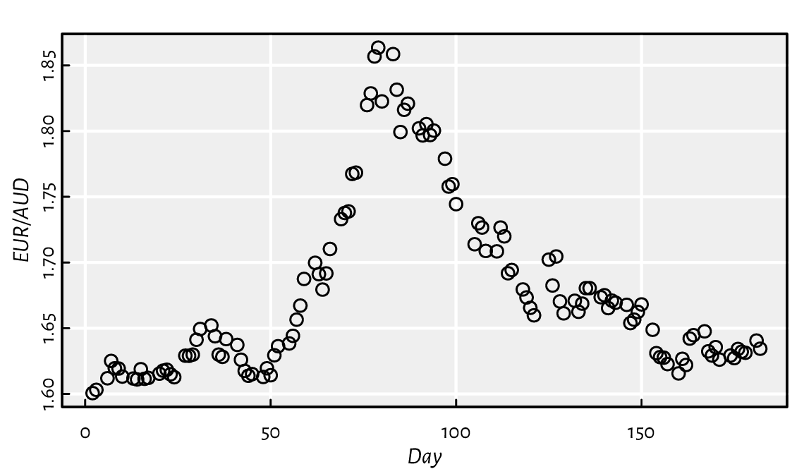
Figure 2.1 EUR/AUD exchange rates from 2020-01-01 (day 1) to 2020-06-30 (day 182).

Somewhat misleadingly (and for reasons that will become apparent later), the documentation of plot can be accessed by calling help("plot.default"). Read about, and experiment with, different values of the main, xlab, ylab, type, col, pch, cex, lty, and lwd arguments. More plotting routines will be discussed in Chapter 13.

2.2. Creating named objects

The objects we bring forth will often need to be memorised so that they can be referred to in further computations. The assignment operator, `<-`, can be used for this purpose:

x <- 1:3  # creates a numeric vector and binds the name `x` to it

The now-named object can be recalled[4] and dealt with as we please:

print(x)  # or just `x` in the R console
## [1] 1 2 3
sum(x)    # example operation: compute the sum of all elements in `x`
## [1] 6

Important

In R, all names are case-sensitive. Hence, x and X can coexist peacefully: when set, they refer to two different objects. If we tried calling Print(x), print(X), or PRINT(x), we would get an error.

Typically, we will be using syntactic names. In help("make.names"), we read: A syntactically valid name consists of letters, numbers and the dot or underline characters and starts with a letter or the dot not followed by a number. Names such as .2way are not valid, and neither are the reserved words such as if, for, function, next, and TRUE, but see Section 9.3.1 for an exception.

A fine name is self-explanatory and thus reader-friendly: patients, mean, and average_scores are way better (if they are what they claim they are) than xyz123, crap, or spam. Also, it might not be such a bad idea to get used to denoting:

• vectors by x, y, z,

• matrices (and matrix-like objects) by A, B, …, X, Y, Z,

• integer indexes by letters i, j, k, l,

• object sizes by n, m, d, p or nx, ny, etc.,

especially when they are only of temporary nature (for storing auxiliary results, iterating over collections of objects, etc.).

There are numerous naming conventions that we can adopt, but most often they are a matter of taste; snake_case, lowerCamelCase, UpperCamelCase, flatcase, or dot.case are equally sound as long as they are used coherently (for instance, some use snake_case for vectors and UpperCamelCase for functions). Occasionally, we have little choice but to adhere to the naming conventions of the project we are about to contribute to.

Note

Generally, a dot, “.”, has no special meaning[5]; na.omit is as appropriate a name as na_omit, naOmit, NAOMIT, naomit, and NaOmit. Readers who know other programming languages will need to habituate themselves to this convention.

R, as a dynamic language, allows for introducing new variables at any time. Moreover, existing names can be bound to new values. For instance:

(y <- "spam")  # bracketed expression – printing not suppressed
## [1] "spam"
x <- y  # overwrites the previous `x`
print(x)
## [1] "spam"

Now x refers to a verbatim copy of y.

Note

Objects are automatically destroyed when we cannot access them anymore. By now, the garbage collector is likely to have got rid of the foregoing 1:3 vector (to which the name x was bound previously).

2.3. Vectorised mathematical functions

Mathematically, we will be denoting a given vector \(\boldsymbol{x}\) of length \(n\) by \((x_1, x_2, \dots, x_n)\). In other words, \(x_i\) is its \(i\)-th element. Let’s review a few operations that are ubiquitous in numerical computing.

2.3.1. abs and sqrt

R implements vectorised versions of the most popular mathematical functions, e.g., abs (absolute value, \(|x|\)) and sqrt (square root, \(\sqrt{x}\)).

abs(c(2, -1, 0, -3, NA_real_))
## [1]  2  1  0  3 NA

Here, vectorised means that instead of being defined to act on a single numeric value, they are applied on each element in a vector. The \(i\)-th resulting item is a transformed version of the \(i\)-th input:

\[ |\boldsymbol{x}| = (|x_1|, |x_2|, \dots, |x_n|). \]

Moreover, if an input is a missing value, the corresponding output will be marked as unknown as well.

Another example:

x <- c(4, 2, -1)
(y <- sqrt(x))
## Warning in sqrt(x): NaNs produced
## [1] 2.0000 1.4142    NaN

To attract our attention to the fact that computing the square root of a negative value is a reckless act, R generated an informative warning. However, a warning is not an error: the result is being produced as usual. In this case, the ill value is marked as not-a-number.

Also, the fact that the irrational \(\sqrt{2}\) is displayed[6] as 1.4142 does not mean that it is such a crude approximation to \(1.414213562373095048801688724209698...\). It was rounded when printing purely for aesthetic reasons. In fact, in Section 3.2.3, we will point out that the computer’s floating-point arithmetic has roughly 16 decimal digits precision (but we shall see that the devil is in the detail).

print(y, digits=16)  # display more significant figures
## [1] 2.000000000000000 1.414213562373095               NaN

2.3.2. Rounding

The following functions drop all or portions of fractional parts of numbers:

• floor(x) (rounds down to the nearest integer, denoted \(\lfloor x\rfloor\)),

• ceiling(x) (rounds up, denoted \(\lceil x\rceil=-\lfloor -x\rfloor\)),

• trunc(x) (rounds towards zero),

• round(x, digits=0) (rounds to the nearest number with digits decimal digits).

For instance:

x <- c(7.0001, 6.9999, -4.3149, -5.19999, 123.4567, -765.4321, 0.5, 1.5, 2.5)
floor(x)
## [1]    7    6   -5   -6  123 -766    0    1    2
ceiling(x)
## [1]    8    7   -4   -5  124 -765    1    2    3
trunc(x)
## [1]    7    6   -4   -5  123 -765    0    1    2

Note

When we write that a function’s usage is like round(x, digits=0), compare help("round"), we mean that the digits parameter is equipped with the default value of 0. In other words, if rounding to 0 decimal digits is what we need, the second argument can be omitted.

round(x)  # the same as round(x, 0); round half to even
## [1]    7    7   -4   -5  123 -765    0    2    2
round(x, 1)  # round to tenths (nearest 0.1s)
## [1]    7.0    7.0   -4.3   -5.2  123.5 -765.4    0.5    1.5    2.5
round(x, -2)  # round to hundreds (nearest 100s)
## [1]    0    0    0    0  100 -800    0    0    0

2.3.3. Natural exponential function and logarithm

Moreover:

• exp(x) outputs the natural exponential function, \(e^x\), where Euler’s number \(e\simeq 2.718\),

• log(x, base=exp(1)) computes, by default, the natural logarithm of \(x\), \(\log_e x\) (which is most often denoted simply by \(\log x\)).

Recall that if \(x=e^y\), then \(\log_e x = y\), i.e., one is the inverse of the other.

log(c(0, 1, 2.7183, 7.3891, 20.0855))  # grows slowly
## [1] -Inf    0    1    2    3
exp(c(0, 1, 2, 3))                     # grows fast
## [1]  1.0000  2.7183  7.3891 20.0855

These functions enjoy a number of very valuable identities and inequalities. In particular, we should know from school that \(\log(x\cdot y)=\log x + \log y\), \(\log(x^y) = y\log x\), and \(e^{x+y} = e^x\cdot e^y\).

For the logarithm to a different base, say, \(\log_{10} x\), we can call:

log(c(0, 1, 10, 100, 1000, 1e10), 10)  # or log(..., base=10)
## [1] -Inf    0    1    2    3   10

Recall that if \(\log_{b} x=y\), then \(x=b^y\), for any \(1\neq b>0\).

Example 2.4

Commonly, a logarithmic scale is used for variables that grow rapidly when expressed as functions of each other; see Figure 2.2.

x <- seq(0, 10, length.out=1001)
par(mfrow=c(1, 2))  # two plots in one figure (one row, two columns)
plot(x, exp(x), type="l")  # left subplot
plot(x, exp(x), type="l", log="y")  # log-scale on the y-axis; right subplot

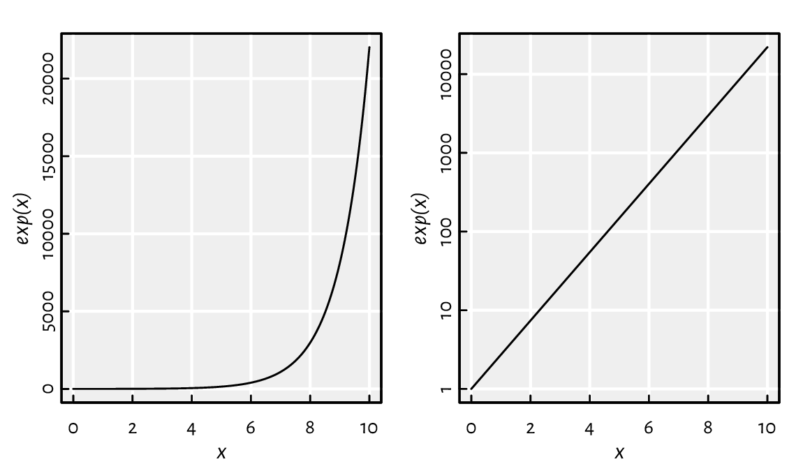
Figure 2.2 Linear- vs log-scale on the y-axis.

Let’s highlight that \(e^x\) on the log-scale is nothing more than a straight line. Such a transformation of the axes can only be applied in the case of values strictly greater than 0.

2.3.4. Probability distributions (*)

It should come as no surprise that R offers extensive support for many univariate probability distribution families, including:

• continuous distributions, i.e., those whose support is comprised of uncountably many real numbers (e.g., some interval or the whole real line):

  • *unif (uniform),

  • *norm (normal),

  • *exp (exponential),

  • *gamma (gamma, \(\Gamma\)),

  • *beta (beta, \(\mathrm{B}\)),

  • *lnorm (log-normal),

  • *t (Student),

  • *cauchy (Cauchy–Lorentz),

  • *chisq (chi-squared, \(\chi^2\)),

  • *f (Snedecor–Fisher),

  • *weibull (Weibull);

  with the prefix “*” being one of:

  • d (probability density function, PDF),

  • p (cumulative distribution function, CDF; or survival function, SF),

  • q (quantile function, being the inverse of the CDF),

  • r (generation of random deviates; already mentioned above);

• discrete distributions, i.e., those whose possible outcomes can easily be enumerated (e.g., some integers):

  • *binom (binomial),

  • *geom (geometric),

  • *pois (Poisson),

  • *hyper (hypergeometric),

  • *nbinom (negative binomial);

  prefixes “p” and “r” retain their meaning, however:

  • d now gives the probability mass function (PMF),

  • q brings about the quantile function, defined as a generalised inverse of the CDF.

Each distribution is characterised by a set of underlying parameters. For instance, a normal distribution \(\mathrm{N}(\mu, \sigma)\) can be pinpointed by setting its expected value \(\mu\in\mathbb{R}\) and standard deviation \(\sigma>0\). In R, these two have been named mean and sd, respectively; see help("dnorm"). Therefore, e.g., dnorm(x, 1, 2) computes the PDF of \(\mathrm{N}(1, 2)\) at x.

Note

The parametrisations assumed in R can be subtly different from what we know from statistical textbooks or probability courses. For example, the normal distribution can be identified based on either standard deviation or variance, and the exponential distribution can be defined via expected value or its reciprocal. We thus advise the reader to study carefully the documentation of help("dnorm"), help("dunif"), help("dexp"), help("dbinom"), and the like.

It is also worth knowing the typical use cases of each of the distributions listed, e.g., a Poisson distribution can describe the probability of observing the number of independent events in a fixed time interval (e.g., the number of users downloading a copy of R from CRAN per hour), and an exponential distribution can model the time between such events; compare [23].

Exercise 2.5

A call to hist(x) draws a histogram, which can serve as an estimator of the underlying continuous probability density function of a given sample; see Figure 2.3 for an illustration.

par(mfrow=c(1, 2))  # two plots in one figure
# left subplot: uniform U(0, 1)
hist(runif(10000, 0, 1), col="white", probability=TRUE, main="")
x <- seq(0, 1, length.out=101)
lines(x, dunif(x, 0, 1), lwd=2)  # draw the true density function (PDF)
# right subplot: normal N(0, 1)
hist(rnorm(10000, 0, 1), col="white", probability=TRUE, main="")
x <- seq(-4, 4, length.out=101)
lines(x, dnorm(x, 0, 1), lwd=2)  # draw the PDF

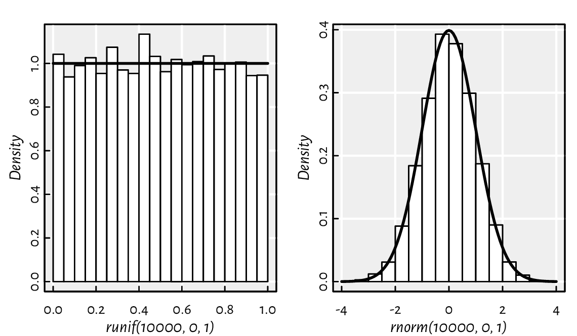
Figure 2.3 Example histograms of some pseudorandom samples and the true underlying probability density functions: the uniform distribution on the unit interval (left) and the standard normal distribution (right).

Draw a histogram of some random samples of different sizes n from the following distributions:

• rnorm(n, µ, σ) – normal \(\mathrm{N}(\mu, \sigma)\) with expected values \(\mu\in\{-1, 0, 5\}\) (i.e., \(\mu\) being equal to either \(-1\), \(0\), or \(5\); read “\(\in\)” as “belongs to the given set” or “in”) and standard deviations \(\sigma\in\{0.5, 1, 5\}\);

• runif(n, a, b) – uniform \(\mathrm{U}(a, b)\) on the interval \((a, b)\) with \(a=0\) and \(b=1\) as well as \(a=-1\) and \(b=1\);

• rbeta(n, α, β) – beta \(\mathrm{B}(\alpha, \beta)\) with \(\alpha,\beta\in\{0.5, 1, 2\}\);

• rexp(n, λ) – exponential \(\mathrm{E}(\lambda)\) with rates \(\lambda\in\{0.5, 1, 10\}\);

Moreover, read about and play with the breaks, main, xlab, ylab, xlim, ylim, and col parameters; see help("hist").

Example 2.6

We roll a six-sided dice twelve times. Let \(C\) be a random variable describing the number of cases where the “1” face is thrown. \(C\) follows a binomial distribution \(\mathrm{Bin}(n, p)\) with parameters \(n=12\) (the number of Bernoulli trials) and \(p=1/6\) (the probability of success in a single roll).

The probability mass function, dbinom, represents the probabilities that the number of “1”s rolled is equal to \(0\), \(1\), …, or \(12\), i.e., \(P(C=0)\), \(P(C=1)\), …, or \(P(C=12)\), respectively:

round(dbinom(0:12, 12, 1/6), 2)  # PMF at 13 different points
##  [1] 0.11 0.27 0.30 0.20 0.09 0.03 0.01 0.00 0.00 0.00 0.00 0.00 0.00

On the other hand, the probability that we throw no more than three “1”s, \(P(C \le 3)\), can be determined by means of the cumulative distribution function, pbinom:

pbinom(3, 12, 1/6)  # pbinom(3, 12, 1/6, lower.tail=FALSE)
## [1] 0.87482

The smallest \(c\) such that \(P(C \le c)\ge 0.95\) can be computed based on the quantile function:

qbinom(0.95, 12, 1/6)
## [1] 4
pbinom(3:4, 12, 1/6)   # for comparison: 0.95 is in-between
## [1] 0.87482 0.96365

In other words, at least 95% of the time, we will be observing no more than four successes.

Also, here are 30 pseudorandom realisations (simulations) of the random variable \(C\):

rbinom(30, 12, 1/6)  # how many successes in 12 trials, repeated 30 times
##  [1] 1 3 2 4 4 0 2 4 2 2 4 2 3 2 0 4 1 0 1 4 4 3 2 6 2 3 2 2 1 1

2.3.5. Special functions (*)

Within mathematical formulae and across assorted application areas, certain functions appear more frequently than others. Hence, for the sake of notational brevity and computational precision, many of them have been assigned special names. For instance, the following functions are mentioned in the definitions related to a few probability distributions:

• gamma(x) for \(x>0\) computes \(\Gamma(x) = \int_0^\infty t^{x-1} e^{-t} \,dt\),

• beta(a, b) for \(a,b>0\) yields \(B(a, b) = \frac{\Gamma(a) \Gamma(b)}{\Gamma(a+b)} = \int_0^1 t^{a-1} (1-t)^{b-1}\,dt\).

Why do we have beta if it is merely a mix of gammas? A specific, tailored function is expected to be faster and more precise than its DIY version; its underlying implementation does not have to involve any calls to gamma.

beta(0.25, 250)  # okay
## [1] 0.91213
gamma(0.25)*gamma(250)/gamma(250.25)  # not okay
## [1] NaN

The \(\Gamma\) function grows so rapidly that already gamma(172) gives rise to Inf. It is due to the fact that a computer’s arithmetic is not infinitely precise; compare Section 3.2.3.

Special functions are plentiful; see the open-access NIST Digital Library of Mathematical Functions [51] for one of the most definitive references (and also [2] for its predecessor). R package gsl [33] provides a vectorised interface to the GNU GSL [28] library, which implements many of such routines.

Exercise 2.7

The Pochhammer symbol, \((a)_x = \Gamma(a+x)/\Gamma(a)\), can be computed via a call to gsl::poch(a, x), i.e., the poch function from the gsl package:

# call install.packages("gsl") first
library("gsl")  # load the package
poch(10, 3:6)   # calls gsl_sf_poch() from GNU GSL
## [1]    1320   17160  240240 3603600

Read the documentation of the corresponding gsl_sf_poch function in the GNU GSL manual. And when you are there, do not hesitate to go through the list of all functions, including those related to statistics, permutations, combinations, and so forth.

Many functions also have their logarithm-of versions; see, e.g., lgamma and lbeta. Also, for instance, dnorm and dbeta have the log parameter. Their classical use case is the (numerical) maximum likelihood estimation, which involves the sums of the logarithms of densities.

2.4. Arithmetic operations

2.4.1. Vectorised arithmetic operators

R features the following binary arithmetic operators:

• `+` (addition) and `-` (subtraction),

• `*` (multiplication) and `/` (division),

• `%/%` (integer division) and `%%` (modulo, division remainder),

• `^` (exponentiation; synonym: `**`).

They are all vectorised: they take two vectors on input and produce another vector on output.

c(1, 2, 3) * c(10, 100, 1000)
## [1]   10  200 3000

The operation was performed in an elementwise fashion on the corresponding pairs of elements from both vectors. The first element in the left sequence was multiplied by the corresponding element in the right vector, and the result was stored in the first element of the output. Then, the second element in the left… all right, we get it.

Other operators behave similarly:

0:10 + seq(0, 1, 0.1)
##  [1]  0.0  1.1  2.2  3.3  4.4  5.5  6.6  7.7  8.8  9.9 11.0
0:7 / rep(3, length.out=8)   # division by 3
## [1] 0.00000 0.33333 0.66667 1.00000 1.33333 1.66667 2.00000 2.33333
0:7 %/% rep(3, length.out=8) # integer division
## [1] 0 0 0 1 1 1 2 2
0:7 %% rep(3, length.out=8)  # division remainder
## [1] 0 1 2 0 1 2 0 1

Operations involving missing values also yield NAs:

c(1, NA_real_, 3, NA_real_) + c(NA_real_, 2, 3, NA_real_)
## [1] NA NA  6 NA

2.4.2. Recycling rule

Some of the preceding statements can be written more concisely. When the operands are of different lengths, the shorter one is recycled as many times as necessary, as in rep(y, length.out=length(x)). For example:

0:7 / 3
## [1] 0.00000 0.33333 0.66667 1.00000 1.33333 1.66667 2.00000 2.33333
1:10 * c(-1, 1)
##  [1] -1  2 -3  4 -5  6 -7  8 -9 10
2 ^ (0:10)
##  [1]    1    2    4    8   16   32   64  128  256  512 1024

We call this the recycling rule.

If an operand cannot be recycled in its entirety, a warning[7] is generated, but the output is still available.

c(1, 10, 100) * 1:8
## Warning in c(1, 10, 100) * 1:8: longer object length is not a multiple of
##     shorter object length
## [1]   1  20 300   4  50 600   7  80

Vectorisation and the recycling rule are perhaps most fruitful when applying binary operators on sequences of identical lengths or when performing vector-scalar (i.e., a sequence vs a single value) operations. However, there is much more: schemes like “every \(k\)-th element” appear in Taylor series expansions (multiply by c(-1, 1)), \(k\)-fold cross-validation, etc.; see also Section 11.3.4 for use cases in matrix/tensor processing.

Also, pmin and pmax return the parallel minimum and maximum of the corresponding elements of the input vectors. Their behaviour is the same as the arithmetic operators, but we call them as ordinary functions:

pmin(c(1, 2, 3, 4), c(4, 2, 3, 1))
## [1] 1 2 3 1
pmin(3, 1:5)
## [1] 1 2 3 3 3
pmax(0, pmin(1, c(0.25, -2, 5, -0.5, 0, 1.3, 0.99)))  # clipping to [0, 1]
## [1] 0.25 0.00 1.00 0.00 0.00 1.00 0.99

Note

Some functions can be very deeply vectorised, i.e., with respect to multiple arguments. For example:

runif(3, c(10, 20, 30), c(11, 22, 33))
## [1] 10.288 21.577 31.227

generates three random numbers uniformly distributed over the intervals \((10, 11)\), \((20, 22)\), and \((30, 33)\), respectively.

2.4.3. Operator precedence

Expressions involving multiple operators need a set of rules governing the order of computations (unless we enforce it using round brackets). We have said that -1:10 means (-1):10 rather than -(1:10). But what about, say, 1+1+1+1+1*0 or 3*2^0:5+10?

Let’s list the operators mentioned so far in their order of precedence, from the least to the most binding (see also help("Syntax")):

1. `<-` (right to left),

2. `+` and `-` (binary),

3. `*` and `/`,

4. `%%` and `%/%`,

5. `:`,

6. `+` and `-` (unary),

7. `^` (right to left).

Hence, -2^2/3+3*4 means ((-(2^2))/3)+(3*4) and not, e.g., -((2^(2/(3+3)))*4).

Notice that `+` and `-`, `*` and `/`, as well as `%%` and `%/%` have the same priority. Expressions involving a series of operations in the same group are evaluated left to right, with the exception of `^` and `<-`, which are performed the other way around. Therefore:

• 2*3/4*5 is equivalent to ((2*3)/4)*5,

• 2^3^4 is 2^(3^4) because, mathematically, we would write it as \(2^{3^4}=2^{81}\),

• “x <- y <- 4*3%%8/2” binds both y and x to 6, not x to the previous value of y and then y to 6.

When in doubt, we can always bracket a subexpression to ensure it is executed in the intended order. It can also increase the readability of our code.

2.4.4. Accumulating

The `+` and `*` operators, as well as the pmin and pmax functions, implement elementwise operations that are applied on the corresponding elements taken from two given vectors. For instance:

\[ \left( \begin{array}{c} x_1 \\ x_2 \\ x_3 \\ \vdots \\ x_n \end{array} \right) + \left( \begin{array}{c} y_1 \\ y_2 \\ y_3 \\ \vdots \\ y_n \end{array} \right) = \left( \begin{array}{c} x_1+y_1 \\ x_2+y_2 \\ x_3+y_3 \\ \vdots \\ x_n+y_n \end{array} \right). \]

However, we can also scan through all the values in a single vector and combine the successive elements that we inspect using the corresponding operation:

• cumsum(x) gives the cumulative sum of the elements in a vector,

• cumprod(x) computes the cumulative product,

• cummin(x) yields the cumulative minimum,

• cummax(x) breeds the cumulative maximum.

The \(i\)-th element in the output vector will consist of the sum/product/min/max of the first \(i\) inputs. For example:

\[ \mathrm{cumsum}\left( \begin{array}{c} x_1 \\ x_2 \\ x_3 \\ \vdots \\ x_n \end{array} \right) = \left( \begin{array}{l} x_1 \\ x_1+x_2 \\ x_1+x_2+x_3 \\ \ \vdots\qquad\qquad\quad\ddots \\ x_1+x_2+x_3+\dots+x_n \end{array} \right). \]

cumsum(1:8)
## [1]  1  3  6 10 15 21 28 36
cumprod(1:8)
## [1]     1     2     6    24   120   720  5040 40320
cummin(c(3, 2, 4, 5, 1, 6, 0))
## [1] 3 2 2 2 1 1 0
cummax(c(3, 2, 4, 5, 1, 6, 0))
## [1] 3 3 4 5 5 6 6

Example 2.8

On a side note, diff can be considered an inverse to cumsum. It computes the iterated difference: subtracts the first two elements, then the second from the third one, the third from the fourth, and so on. In other words, diff(x) gives \(\boldsymbol{y}\) such that \(y_i=x_{i+1}-x_i\).

x <- c(-2, 3, 6, 2, 15)
diff(x)
## [1]  5  3 -4 13
cumsum(diff(x))
## [1]  5  8  4 17
cumsum(c(-2, diff(x)))  # recreates x
## [1] -2  3  6  2 15

Thanks to diff, we can compute the daily changes to the EUR/AUD forex rates studied earlier; see Figure 2.4.

aud <- scan(paste0("https://github.com/gagolews/teaching-data/raw/",
    "master/marek/euraud-20200101-20200630.csv"), comment.char="#")
aud_all <- na.omit(aud)  # remove all missing values
plot(diff(aud_all), type="s", ylab="Daily change [EUR/AUD]")  # "steps"
abline(h=0, lty="dotted")  # draw a horizontal line at y=0

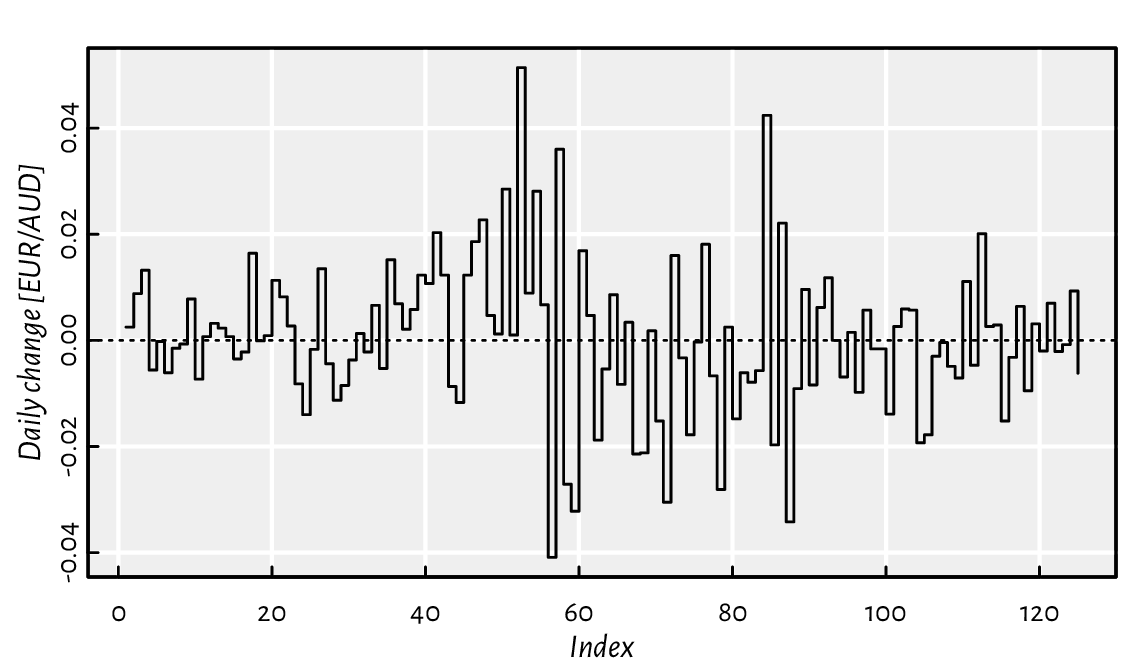
Figure 2.4 Iterated differences of the exchange rates (non-missing values only).

2.4.5. Aggregating

If we are only concerned with the last cumulant, which summarises all the inputs, we have the following[8] functions at our disposal:

• sum(x) computes the sum of elements in a vector, \(\sum_{i=1}^n x_i=x_1+x_2+\cdots+x_n\),

• prod(x) outputs the product of all elements, \(\prod_{i=1}^n x_i=x_1 x_2 \cdots x_n\),

• min(x) determines the minimum,

• max(x) reckons the greatest value.

sum(1:8)
## [1] 36
prod(1:8)
## [1] 40320
min(c(3, 2, 4, 5, 1, 6, 0))
## [1] 0
max(c(3, 2, 4, 5, 1, 6, 0))
## [1] 6

The foregoing functions form the basis for the popular summary statistics[9] (sample aggregates) such as:

• mean(x) gives the arithmetic mean, sum(x)/length(x),

• var(x) yields the (unbiased) sample variance, sum((x-mean(x))^2)/(length(x)-1),

• sd(x) is the standard deviation, sqrt(var(x)).

Furthermore, median(x) computes the sample median, i.e., the middle value in the sorted[10] version of x.

For instance:

x <- runif(1000)
c(min(x), mean(x), median(x), max(x), sd(x))
## [1] 0.00046535 0.49727780 0.48995025 0.99940453 0.28748391

Exercise 2.9

Let \(\boldsymbol{x}\) be any vector of length \(n\) with positive elements. Compute its geometric and harmonic mean, which are given by, respectively,

\[ \sqrt[n]{\prod_{i=1}^n x_i}=e^{\frac{1}{n} \sum_{i=1}^n \log x_i} \quad\text{ and }\quad \frac{n}{\sum_{i=1}^n \frac{1}{x_i}}. \]

When solving exercises like this one, it does not really matter what data you apply these functions on. We are being abstract in the sense that the \(\boldsymbol{x}\) vector can be anything: from the one that features very accurate socioeconomic predictions that will help make this world less miserable, through the data you have been collecting for the last ten years in relation to your super important PhD research, whatever your company asked you to crunch today, to something related to the hobby project that you enjoy doing after hours. But you can also just test the above on something like “x <- runif(10)”, and move on.

All aggregation functions return a missing value if any of the input elements is unavailable. Luckily, they are equipped with the na.rm parameter, on behalf of which we can request the removal of NAs.

aud <- scan(paste0("https://github.com/gagolews/teaching-data/raw/",
    "master/marek/euraud-20200101-20200630.csv"), comment.char="#")
c(min(aud), mean(aud), max(aud))
## [1] NA NA NA
c(min(aud, na.rm=TRUE), mean(aud, na.rm=TRUE), max(aud, na.rm=TRUE))
## [1] 1.6006 1.6775 1.8635

Otherwise, we could have called, e.g., mean(na.omit(x)).

Note

In the documentation, we read that the usage of sum, prod, min, and max is like sum(..., na.rm=FALSE), etc. In this context, it means that they accept any number of input vectors, and each of them can be of arbitrary length. Therefore, min(1, 2, 3), min(c(1, 2, 3)) as well as min(c(1, 2), 3) all return the same result.

However, we also read that we have mean(x, trim=0, na.rm=FALSE, ...). This time, only one vector can be aggregated, and any further arguments (except trim and na.rm) are ignored.

The extra flexibility (which we do not have to rely on, ever) of the former group is due to their being associative operations. We have, e.g., \((2+3)+4 = 2+(3+4)\). Hence, these operations can be performed in any order, in any group. They are primitive operations: it is mean that is based on sum, not vice versa.

2.5. Exercises

Exercise 2.10

Answer the following questions.

• What is the meaning of the dot-dot-dot parameter in the definition of the c function?

• We say that the round function is vectorised. What does that mean?

• What is wrong with a call to c(sqrt(1), sqrt(2), sqrt(3))?

• What do we mean by saying that multiplication operates element by element?

• How does the recycling rule work when applying `+`?

• How to (and why) set the seed of the pseudorandom number generator?

• What is the difference between NA_real_ and NaN?

• How are default arguments specified in the manual of, e.g., the round function?

• Is a call to rep(times=4, x=1:5) equivalent to rep(4, 1:5)?

• List a few ways to generate a sequence like (-1, -0.75, -0.5, …, 0.75, 1).

• Is -3:5 the same as -(3:5)? What about the precedence of operators in expressions such as 2^3/4*5^6, 5*6+4/17%%8, and 1+-2^3:4-1?

• If x is a numeric vector of length \(n\) (for some \(n\ge 0\)), how many values will sample(x) output?

• Does scan support reading directly from compressed archives, e.g., .csv.gz files?

When in doubt, refer back to the material discussed in this chapter or the R manual.

Exercise 2.11

Thanks to vectorisation, implementing an example graph of arcsine and arccosine is straightforward.

x <- seq(-1, 1, length.out=11)  # increase length.out for a smoother curve
plot(x, asin(x),                # asin() computed for 11 points
    type="l",                   # lines
    ylim=c(-pi/2, pi),          # y axis limits like c(y_min, y_max)
    ylab="asin(x), acos(x)")    # y axis label
lines(x, acos(x), col="red", lty="dashed")  # adds to the current plot
legend("topright", c("asin(x)", "acos(x)"),
    lty=c("solid", "dashed"), col=c("black", "red"), bg="white")

Thusly inspired, plot the following functions: \(|\sin x^2|\), \(\left|\sin |x|\right|\), \(\sqrt{\lfloor x\rfloor}\), and \(1/(1+e^{-x})\). Recall that the documentation of plot can be accessed by calling help("plot.default").

Exercise 2.12

The expression:

\[ 4 \sum_{i=1}^n \frac{(-1)^{i+1}}{2i-1} = 4\left( \frac{1}{1} - \frac{1}{3} + \frac{1}{5} - \frac{1}{7} + \cdots \right) \]

slowly converges to \(\pi\) as \(n\) approaches \(\infty\). Calculate it for \(n=1 000 000\) and \(n=1 000 000 000\) using the vectorised functions and operators discussed in this chapter, making use of the recycling rule as much as possible.

Exercise 2.13

Let x and y be two vectors of identical lengths \(n\), say:

x <- rnorm(100)
y <- 2*x+10+rnorm(100, 0, 0.5)

Compute the Pearson linear correlation coefficient given by:

\[ r = \frac{ \sum_{i=1}^n \left(x_i-\frac{1}{n}\sum_{j=1}^n x_j \right) \left(y_i-\frac{1}{n}\sum_{j=1}^n y_j \right) }{ \sqrt{\sum_{i=1}^n \left(x_i-\frac{1}{n}\sum_{j=1}^n x_j \right)^2}\, \sqrt{\sum_{i=1}^n \left(y_i-\frac{1}{n}\sum_{j=1}^n y_j \right)^2} }. \]

To make sure you have come up with a correct implementation, compare your result to a call to cor(x, y).

Exercise 2.14

(*) Find an R package providing a function to compute moving (rolling) averages and medians of a given vector. Apply them on the EUR/AUD currency exchange data. Draw thus obtained smoothened versions of the time series.

Exercise 2.15

(**) Use a call to convolve(..., type="filter") to compute the \(k\)-moving average of a numeric vector.

In the next chapter, we will study operations that involve logical values.

---

[1]

A dot has no special meaning in R; see Section 2.2.

[2]

Some “caring” R users might be tempted to introduce two new functions now, one for generating (1, 2, 3, 1, 2, 3, …) only and the other outputting patterns like (1, 1, 1, 2, 2, 2, …). They would most likely wrap them in a new package and announce that on social media. But this is nothing else than a multiplication of entities without actual necessity. This way, we would end up with three functions. First is the original one, rep, which everyone ought to know anyway because it is part of the standard library. Second and third are the two redundant procedures whose user-friendliness is only illusory. See also Chapter 9 for a discussion on the design of functions.

[3]

Certain configurations of seq and its variants might return vectors of the type integer instead of double, some of them in a compact (ALTREP) form; see Section 6.4.1.

[4]

Name bindings are part of environment frames; see Chapter 16.

[5]

See Section 10.2 and Section 16.2.1 for a few asterisks.

[6]

There are a couple of settings in place that control the default behaviour of the print function; see width, digits, max.print, OutDec, scipen, etc. in help("options").

[7]

A few functions do not warn us whatsoever when they perform incomplete recycling (e.g., paste) or can even give an error (e.g., as.data.frame.list). Consider this inconsistency an annoying bug and hope it will be fixed, in the next decade or so.

[8]

Chapter 7 will discuss the Reduce function, which generalises the above by allowing any binary operation to be propagated over a given vector.

[9]

Actually, var and median, amongst others, are defined by the stats package. But this one is automatically loaded by default, so let’s not make a fuss about it now.

[10]

min, median, and max are generalised by the quantile function. We will discuss it much later (Section 4.4.3), because it returns a named vector.