3. Logical vectors
This open-access textbook is, and will remain, freely available for everyone’s enjoyment (also in PDF; a paper copy can also be ordered). It is a non-profit project. Although available online, it is a whole course, and should be read from the beginning to the end. Refer to the Preface for general introductory remarks. Any bug/typo reports/fixes are appreciated. Make sure to check out Minimalist Data Wrangling with Python [28], too.
3.1. Creating logical vectors
R defines three(!) logical constants: TRUE, FALSE, and NA
representing, respectively, “yes”, “no”, and “???”.
When instantiated, each of them is an atomic vector of length one.
To generate logical vectors of arbitrary size, we can call
some of the functions introduced in the previous chapter, for instance:
c(TRUE, FALSE, FALSE, NA, TRUE, FALSE)
## [1]  TRUE FALSE FALSE    NA  TRUE FALSE
rep(c(TRUE, FALSE, NA), each=2)
## [1]  TRUE  TRUE FALSE FALSE    NA    NA
sample(c(TRUE, FALSE), 10, replace=TRUE, prob=c(0.8, 0.2))
##  [1]  TRUE  TRUE  TRUE FALSE FALSE  TRUE  TRUE FALSE  TRUE  TRUE
Note
By default, T is a synonym for TRUE and F stands for FALSE.
However, these are not reserved keywords and can be reassigned
to any other values. Therefore, we advise against relying on them:
they are not used throughout the course of this course.
Also, notice that the logical missing value is spelled simply
as NA, and not NA_logical_. Both the logical NA
and the numeric NA_real_
are, for the sake of our widely-conceived wellbeing,
both printed as “NA” on the R console.
This, however, does not mean they are identical;
see Section 4.1 for discussion.
3.2. Comparing elements
3.2.1. Vectorised relational operators
Logical vectors frequently come into being as a result of various testing activities. In particular, the binary operators:
`<` (less than),
`<=` (less than or equal),
`>` (greater than),
`>=` (greater than or equal)
`==` (equal),
`!=` (not equal),
compare the corresponding elements of two numeric vectors and output a logical vector.
1 < 3
## [1] TRUE
c(1, 2, 3, 4) == c(2, 2, 3, 8)
## [1] FALSE  TRUE  TRUE FALSE
1:10 <= 10:1
##  [1]  TRUE  TRUE  TRUE  TRUE  TRUE FALSE FALSE FALSE FALSE FALSE
Thus, they operate in an elementwise manner. Moreover, the recycling rule is applied if necessary:
3 < 1:5  # c(3, 3, 3, 3, 3) < c(1, 2, 3, 4, 5)
## [1] FALSE FALSE FALSE  TRUE  TRUE
c(1, 4) == 1:4  # c(1, 4, 1, 4) == c(1, 2, 3, 4)
## [1]  TRUE FALSE FALSE  TRUE
Therefore, we can say that they are vectorised in the same manner as the arithmetic operators `+`, `*`, etc.; compare Section 2.4.1.
3.2.2. Testing for NA, NaN, and Inf
Comparisons against missing values and not-numbers yield NAs.
Instead of the incorrect “x == NA_real_”,
testing for missingness should rather be performed via a call
to the vectorised is.na function.
is.na(c(NA_real_, Inf, -Inf, NaN, -1, 0, 1))
## [1]  TRUE FALSE FALSE  TRUE FALSE FALSE FALSE
is.na(c(TRUE, FALSE, NA, TRUE))  # works for logical vectors, too
## [1] FALSE FALSE  TRUE FALSE
Moreover, is.finite is noteworthy
since it returns FALSE on Infs, NA_real_s and NaNs.
is.finite(c(NA_real_, Inf, -Inf, NaN, -1, 0, 1))
## [1] FALSE FALSE FALSE FALSE  TRUE  TRUE  TRUE
See also the more specific is.nan and is.infinite.
3.2.3. Dealing with round-off errors (*)
In mathematics, real numbers are merely an idealisation. In practice, however, it is impossible to store them with infinite precision (think \(\pi=3.141592653589793...\)): computer memory is limited, and our time is precious.
Therefore, a consensus had to be reached. In R, we rely on the double-precision floating point format. The floating point part means that the numbers can be both small (close to zero like \(\pm 2.23\times 10^{-308}\)) and large (e.g., \(\pm 1.79\times 10^{308}\)).
Note
2.23e-308 == 0.00000000000000000000000000000000000000000000000000
               00000000000000000000000000000000000000000000000000
               00000000000000000000000000000000000000000000000000
               00000000000000000000000000000000000000000000000000
               00000000000000000000000000000000000000000000000000
               00000000000000000000000000000000000000000000000000
               0000000223

1.79e308  ==                                            179000000
               00000000000000000000000000000000000000000000000000
               00000000000000000000000000000000000000000000000000
               00000000000000000000000000000000000000000000000000
               00000000000000000000000000000000000000000000000000
               00000000000000000000000000000000000000000000000000
               00000000000000000000000000000000000000000000000000
These two are pretty distant.
Every numeric value takes 8 bytes (or, equivalently, 64 bits) of memory. We are, however, able to store only about 15–17 decimal digits:
print(0.12345678901234567890123456789012345678901234, digits=22)  # 22 is max
## [1] 0.1234567890123456773699
which limits the precision of our computations. We wrote about because, unfortunately, the numbers are stored the computer-friendly binary base, not the human-aligned decimal one. This can lead to counterintuitive outcomes. In particular:
0.1cannot be represented exactly for it cannot be written as a finite series of reciprocals of powers of 2 (we have \(0.1=2^{-4}+2^{-5}+2^{-8}+2^{-9}+\dots\)). This leads to surprising results such as:0.1 + 0.1 + 0.1 == 0.3 ## [1] FALSE
Quite strikingly, what follows does not show anything suspicious:
c(0.1, 0.1 + 0.1 + 0.1, 0.3)
## [1] 0.1 0.3 0.3
Printing involves rounding. In the above context, it is misleading. Actually, we experience something more like:
print(c(0.1, 0.1 + 0.1 + 0.1, 0.3), digits=22)
## [1] 0.1000000000000000055511 0.3000000000000000444089
## [3] 0.2999999999999999888978
All integers between \(-2^{53}\) and \(2^{53}\) all stored exactly. This is good news. However, the next integer is beyond the representable range:
2^53 + 1 == 2^53
## [1] TRUE
The order of operations may matter. In particular, the associativity property can be violated when dealing with numbers of contrasting orders of magnitude:
2^53 + 2^-53 - 2^53 - 2^-53  # should be == 0.0
## [1] -1.1102e-16
Some numbers may just be too large, too small, or too close to zero to be represented exactly:
c(sum(2^((1023-52):1023)), sum(2^((1023-53):1023)))
## [1] 1.7977e+308         Inf
c(2^(-1022-52), 2^(-1022-53))
## [1] 4.9407e-324  0.0000e+00
Important
The double-precision floating point format (IEEE 754) is not specific to R. It is used by most other computing environments, including Python and C++. For discussion, see [33, 36, 43], and the more statistically-orientated [31].
Can we do anything about these issues?
Firstly, dealing with integers of a reasonable order of magnitude (e.g., various resource or case IDs in our datasets) is safe. Their comparison, addition, subtraction, and multiplication are always precise.
In all other cases (including applying other operations on integers, e.g., division or sqrt), we need to be very careful with comparisons, especially involving testing for equality via `==`. The sole fact that \(\sin \pi = 0\), mathematically speaking, does not mean that we should expect that:
sin(pi) == 0
## [1] FALSE
Instead, they are so close that we can treat the difference between them as negligible. Thus, in practice, instead of testing if \(x = y\), we will be considering:
\(|x-y|\) (absolute error), or
\(\frac{|x-y|}{|y|}\) (relative error; which takes the order of magnitude of the numbers into account but obviously cannot be applied if \(y\) is very close to \(0\)),
and determining if these are less than an assumed error margin, \(\varepsilon>0\), say, \(10^{-8}\) or \(2^{-26}\). For example:
abs(sin(pi) - 0) < 2^-26
## [1] TRUE
Note
Rounding can sometimes have a similar effect as testing for almost equality in terms of the absolute error.
round(sin(pi), 8) == 0
## [1] TRUE
Important
The foregoing recommendations are valid for the most popular applications of R, i.e., statistical and, more generally, scientific computing[1]. Our datasets usually do not represent accurate measurements. Bah, the world itself is far from ideal! Therefore, we do not have to lose sleep over our not being able to precisely pinpoint the exact solutions.
3.3. Logical operations
3.3.1. Vectorised logical operators
The relational operators such as `==` and `>`
accept only two arguments. Their chaining is forbidden.
A test that we would mathematically write
as \(0 \le x \le 1\) (or \(x\in[0, 1]\)) cannot be expressed
as “0 <= x <= 1” in R.
Therefore, we need a way to combine two logical conditions
so as to be able to state that “\(x\ge 0\) and, at the same time, \(x\le 1\)”.
In such situations, the following logical operators and functions come in handy:
`!` (not, negation; unary),
`&` (and, conjunction; are both predicates true?),
`|` (or, alternation; is at least one true?),
xor (exclusive-or, exclusive disjunction, either-or; is one and only one of the predicates true?).
They again act elementwisely and implement the recycling rule if necessary (and applicable).
x <- c(-10, -1, -0.25, 0, 0.5, 1, 5, 100)
(x >= 0) & (x <= 1)
## [1] FALSE FALSE FALSE  TRUE  TRUE  TRUE FALSE FALSE
(x < 0) | (x > 1)
## [1]  TRUE  TRUE  TRUE FALSE FALSE FALSE  TRUE  TRUE
!((x < 0) | (x > 1))
## [1] FALSE FALSE FALSE  TRUE  TRUE  TRUE FALSE FALSE
xor(x >= -1, x <= 1)
## [1]  TRUE FALSE FALSE FALSE FALSE FALSE  TRUE  TRUE
Important
The vectorised `&` and `|` operators should not be confused with their scalar, short-circuit counterparts, `&&` and `||`; see Section 8.1.4.
3.3.2. Operator precedence revisited
The operators introduced in this chapter have lower precedence than the
arithmetic ones, including the binary `+`
and `-`. Calling help("Syntax") reveals
that we can extend our listing from Section 2.4.3
as follows:
`<-` (right to left; least binding),
`|`,
`&`,
`!` (unary),
`<`, `>`, `<=`, `>=`, `==`, and `!=`,
`+` and `-` (binary),
`*` and `/`,
…
The order of precedence is intuitive,
e.g., “x+1 <= y & y <= z-1 | x <= z”
means “(((x+1) <= y) & (y <= (z-1))) | (x <= z)”.
3.3.3. Dealing with missingness
Operations involving missing values follow the principles
of Łukasiewicz’s three-valued logic, which is based on common sense.
For instance, “NA | TRUE” is TRUE because
the alternative (or) needs at least one
argument to be TRUE to generate a positive result.
On the other hand, “NA | FALSE” is NA since
the outcome would be different depending on what we substituted NA for.
Let’s contemplate the logical operations’ truth tables for all the possible combinations of inputs:
u <- c(TRUE, FALSE, NA,  TRUE,  FALSE, NA,    TRUE, FALSE, NA)
v <- c(TRUE, TRUE, TRUE, FALSE, FALSE, FALSE, NA,   NA,    NA)
!u
## [1] FALSE  TRUE    NA FALSE  TRUE    NA FALSE  TRUE    NA
u & v
## [1]  TRUE FALSE    NA FALSE FALSE FALSE    NA FALSE    NA
u | v
## [1]  TRUE  TRUE  TRUE  TRUE FALSE    NA  TRUE    NA    NA
xor(u, v)
## [1] FALSE  TRUE    NA  TRUE FALSE    NA    NA    NA    NA
3.3.4. Aggregating with all, any, and sum
Just like in the case of numeric vectors,
we can summarise the contents of logical sequences.
all tests whether every element in a logical vector
is equal to TRUE. any determines if there exists
an element that is TRUE.
x <- runif(10000)
all(x <= 0.2)  # are all values in x <= 0.2?
## [1] FALSE
any(x <= 0.2)  # is there at least one element in x that is <= 0.2?
## [1] TRUE
any(c(NA, FALSE, TRUE))
## [1] TRUE
all(c(TRUE, TRUE, NA))
## [1] NA
Note
all will frequently be used in conjunction with `==` as the latter is itself vectorised: it does not test whether a vector as a whole is equal to another one.
z <- c(1, 2, 3)
z == 1:3  # elementwise equal
## [1] TRUE TRUE TRUE
all(z == 1:3)  # elementwise equal summarised
## [1] TRUE
However, let’s keep in mind the warning about the testing for exact equality of floating-point numbers stated in Section 3.2.3. Sometimes, considering absolute or relative errors might be more appropriate.
z <- sin((0:10)*pi)  # sin(0), sin(pi), sin(2*pi), ..., sin(10*pi)
all(z == 0.0)  # danger zone! please don't...
## [1] FALSE
all(abs(z - 0.0) < 1e-8)  # are the absolute errors negligible?
## [1] TRUE
We can also call sum on a logical vector.
Taking into account that it interprets TRUE as numeric 1
and FALSE as 0 (more on this in Section 4.1),
it will give us the number of elements equal to TRUE.
sum(x <= 0.2)  # how many elements in x are <= 0.2?
## [1] 1998
Also, by computing sum(x)/length(x),
we can obtain the proportion (fraction) of values equal to TRUE in x.
Equivalently:
mean(x <= 0.2)  # proportion of elements <= 0.2
## [1] 0.1998
Naturally, we expect
mean(runif(n) <= 0.2) to be equal to
0.2 (20%), but with randomness, we can never be sure.
3.3.5. Simplifying predicates
Each aspiring programmer needs to become fluent with the rules
governing the transformations of logical conditions,
e.g., that the negation of “(x >= 0) & (x < 1)”
is equivalent to “(x < 0) | (x >= 1)”.
Such rules are called tautologies. Here are a few of them:
!(!p)is equivalent top(double negation),!(p & q)holds if and only if!p | !q(De Morgan’s law),!(p | q)is!p & !q(another De Morgan’s law),all
(p)is equivalent to!any(!p).
Various combinations thereof are, of course, possible. Further simplifications are enabled by other properties of the binary operations:
commutativity (symmetry), e.g., \(a+b = b+a\), \(a*b=b*a\),
associativity, e.g., \((a+b)+c = a+(b+c)\), \(\max(\max(a, b), c)=\max(a, \max(b, c))\),
distributivity, e.g., \(a*b+a*c = a*(b+c)\), \(\min(\max(a,b), \max(a,c))=\max(a, \min(b, c))\),
and relations, including:
transitivity, e.g., if \(a\le b\) and \(b\le c\), then surely \(a \le c\).
Assuming that a, b, and c are numeric vectors,
simplify the following expressions:
!(b>a & b<c),!(a>=b & b>=c & a>=c),a>b & a<c | a<c & a>b,a>b | a<=b,a<=b & a>c | a>b & a<=c,a<=b & (a>c | a>b) & a<=c,!all(a > b & b < c).
3.4. Choosing elements with ifelse
The ifelse function is a vectorised version of the scalar
if…else conditional statement, which we will forgo
for as long as until Chapter 8. It permits us to select an element
from one of two vectors based on some logical condition. A call to
ifelse(l, t, f), where l is a logical vector,
returns a vector y such that:
In other words, the \(i\)-th element of the result vector
is equal to \(t_i\) if \(l_i\) is TRUE and to \(f_i\) otherwise.
For example:
(z <- rnorm(6))  # example vector
## [1] -0.560476 -0.230177  1.558708  0.070508  0.129288  1.715065
ifelse(z >= 0, z, -z)  # like abs(z)
## [1] 0.560476 0.230177 1.558708 0.070508 0.129288 1.715065
or:
(x <- rnorm(6))  # example vector
## [1]  0.46092 -1.26506 -0.68685 -0.44566  1.22408  0.35981
(y <- rnorm(6))  # example vector
## [1]  0.40077  0.11068 -0.55584  1.78691  0.49785 -1.96662
ifelse(x >= y, x, y)   # like pmax(x, y)
## [1]  0.46092  0.11068 -0.55584  1.78691  1.22408  0.35981
We should not be surprised anymore that the recycling rule is fired up when necessary:
ifelse(x > 0, x^2, 0)  # squares of positive xs and 0 otherwise
## [1] 0.21244 0.00000 0.00000 0.00000 1.49838 0.12947
Note
All arguments are evaluated in their entirety before deciding on which elements are selected. Therefore, the following call generates a warning:
ifelse(z >= 0, log(z), NA_real_)
## Warning in log(z): NaNs produced
## [1]       NA       NA  0.44386 -2.65202 -2.04571  0.53945
This is because, with log(z),
we compute the logarithms of negative values
anyway. To fix this, we can write:
log(ifelse(z >= 0, z, NA_real_))
## [1]       NA       NA  0.44386 -2.65202 -2.04571  0.53945
In case we yearn for an if…else if…else-type expression, the calls to ifelse can naturally be nested.
A version of
pmax(pmax(x, y), z) can be written as:
ifelse(x >= y,
    ifelse(z >= x, z, x),
    ifelse(z >= y, z, y)
)
## [1] 0.46092 0.11068 1.55871 1.78691 1.22408 1.71506
However, determining three intermediate logical vectors is not necessary. We can save one call to `>=` by introducing an auxiliary variable:
xy <- ifelse(x >= y, x, y)
ifelse(z >= xy, z, xy)
## [1] 0.46092 0.11068 1.55871 1.78691 1.22408 1.71506
Figure 3.1 depicts a realisation of the mixture \(Z=0.2 X + 0.8 Y\) of two normal distributions \(X\sim\mathrm{N}(-2, 0.5)\) and \(Y\sim\mathrm{N}(3, 1)\).
n <- 100000
z <- ifelse(runif(n) <= 0.2, rnorm(n, -2, 0.5), rnorm(n, 3, 1))
hist(z, breaks=101, probability=TRUE, main="", col="white")
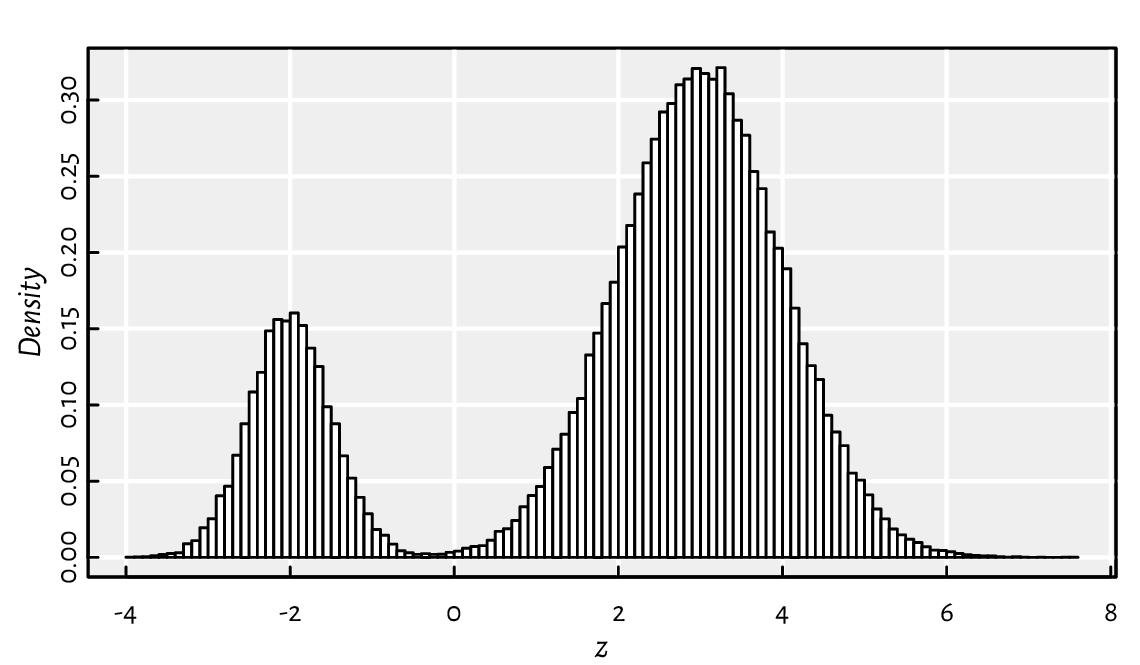
Figure 3.1 A mixture of two Gaussians generated with ifelse.
In other words, we generated a variate from the normal distribution that has the expected value of \(-2\) with probability \(20\%\), and from the one with the expectation of \(3\) otherwise. Thus inspired, generate the Gaussian mixtures:
\(\frac{2}{3} X + \frac{1}{3} Y\), where \(X\sim\mathrm{N}(100, 16)\) and \(Y\sim\mathrm{N}(116, 8)\),
\(0.3 X + 0.4 Y + 0.3 Z\), where \(X\sim\mathrm{N}(-10, 2)\), \(Y\sim\mathrm{N}(0, 2)\), and \(Z\sim\mathrm{N}(10, 2)\).
(*) On a side note, knowing that if \(X\) follows \(\mathrm{N}(0, 1)\), then the scaled-shifted \(\sigma X+\mu\) is distributed \(\mathrm{N}(\mu, \sigma)\), the above can be equivalently written as:
w <- (runif(n) <= 0.2)
z <- rnorm(n, 0, 1)*ifelse(w, 0.5, 1) + ifelse(w, -2, 3)
3.5. Exercises
Answer the following questions.
Why the statement “The Earth is flat or the smallpox vaccine is proven effective” is obviously true?
What is the difference between
NAandNA_real_?Why is “
FALSE & NA” equal toFALSE, but “TRUE & NA” isNA?Why has ifelse
(x>=0,sqrt(x), NA_real_)a tendency to generate warnings and how to rewrite it so as to prevent that from happening?What is the interpretation of mean
(x >= 0 & x <= 1)?For some integer \(x\) and \(y\), how to verify whether \(0 < x < 100\), \(0 < y < 100\), and \(x < y\), all at the same time?
Mathematically, for all real \(x, y > 0\), we have \(\log xy = \log x + \log y\). Why then all
(log(x*y) ==log(x)+log(y))can sometimes returnFALSE? How to fix this?Is
x/y/zalways equal tox/(y/z)? How to fix this?What is the purpose of very specific functions such as log1p and expm1 (see their help page) and many others listed in, e.g., the GNU GSL library [29]? Is our referring to them a violation of the beloved “do not multiply entities without necessity” rule?
If we know that \(x\) may be subject to error, how to test whether \(x>0\) in a robust manner?
Is “
y<-5” the same as “y <- 5” or rather “y < -5”?
What is the difference between all and isTRUE? What about `==`, identical, and all.equal? Is the last one properly vectorised?
Compute the cross-entropy loss between a numeric vector \(\boldsymbol{p}\) with values in the interval \((0, 1)\) and a logical vector \(\boldsymbol{y}\), both of length \(n\) (you can generate them randomly or manually, it does not matter, it is just an exercise):
where
Interpretation: in classification problems,
\(y_i\in\{\text{FALSE}, \text{TRUE}\}\)
denotes the true class of the \(i\)-th object
(say, whether the \(i\)-th hospital patient is symptomatic)
and \(p_i\in(0, 1)\) is a machine learning algorithm’s
confidence that \(i\) belongs to class TRUE
(e.g., how sure a decision tree model is that the corresponding
person is unwell). Ideally, if \(y_i\) is TRUE, \(p_i\) should be close to 1
and to \(0\) otherwise. The cross-entropy loss quantifies by how much
a classifier differs from the omniscient one.
The use of the logarithm penalises strong beliefs in the wrong answer.
By the way, if we have solved any of the exercises encountered so far
by referring to if statements, for loops,
vector indexing like x[...],
or any external R package, we recommend going back and rewrite our code.
Let’s keep things simple (effective, readable)
by only using base R’s vectorised operations that
we have introduced.