11. Matrices and other arrays
This open-access textbook is, and will remain, freely available for everyone’s enjoyment (also in PDF; a paper copy can also be ordered). It is a non-profit project. Although available online, it is a whole course, and should be read from the beginning to the end. Refer to the Preface for general introductory remarks. Any bug/typo reports/fixes are appreciated. Make sure to check out Minimalist Data Wrangling with Python [28], too.
When we equip an atomic or generic vector with the dim attribute,
it automatically becomes an object of the S3 class array.
In particular, two-dimensional arrays (of the primary S3 class matrix)
allow us to represent tabular data where items are aligned into rows
and columns:
structure(1:6, dim=c(2, 3))  # a matrix with two rows and three columns
##      [,1] [,2] [,3]
## [1,]    1    3    5
## [2,]    2    4    6
Combined with the fact that there are many functions overloaded
for the matrix class, we have just opened up a whole world of new
possibilities, which we explore in this chapter.
Namely, we will discuss how to perform the algebraic operations
such as matrix multiplication, transpose, finding eigenvalues,
and performing various decompositions. We will also cover data wrangling
operations such as array subsetting and column- and rowwise aggregation.
Furthermore, the next chapter will present data frames:
matrix-like objects whose columns can be of any (not necessarily
the same) type.
Important
Oftentimes, a numeric matrix with \(n\) rows and \(m\) columns is used to represent \(n\) points (samples, observations) in an \(m\)-dimensional space (with \(m\) numeric features or variables), \(\mathbb{R}^m\).
11.1. Creating arrays
11.1.1. matrix and array
A matrix can be conveniently created using the following function.
(A <- matrix(1:6, byrow=TRUE, nrow=2))
##      [,1] [,2] [,3]
## [1,]    1    2    3
## [2,]    4    5    6
It converted an atomic vector of length six to a matrix with two rows.
The number of columns was determined automatically (ncol=3 could have
been passed, additionally or instead, to get the same result).
Important
By default, the elements of the input vector are read column by column:
matrix(1:6, ncol=3)  # byrow=FALSE
##      [,1] [,2] [,3]
## [1,]    1    3    5
## [2,]    2    4    6
A matrix can be equipped with an attribute that defines dimension names, being a list of two character vectors of appropriate sizes which label each row and column:
matrix(1:6, byrow=TRUE, nrow=2, dimnames=list(c("x", "y"), c("a", "b", "c")))
##   a b c
## x 1 2 3
## y 4 5 6
Alternatively, to create a matrix, we can use the array function. It requires the number of rows and columns to be specified explicitly.
array(1:6, dim=c(2, 3))
##      [,1] [,2] [,3]
## [1,]    1    3    5
## [2,]    2    4    6
The elements were consumed in the column-major order.
Arrays of other dimensionalities are also possible. Here is a one-dimensional array:
array(1:6, dim=6)
## [1] 1 2 3 4 5 6
When printed, it is indistinguishable from an atomic vector
(but the class attribute is still set to array).
And now for something completely different: a three-dimensional array
of size \(3\times 4\times 2\):
array(1:24, dim=c(3, 4, 2))
## , , 1
##
##      [,1] [,2] [,3] [,4]
## [1,]    1    4    7   10
## [2,]    2    5    8   11
## [3,]    3    6    9   12
##
## , , 2
##
##      [,1] [,2] [,3] [,4]
## [1,]   13   16   19   22
## [2,]   14   17   20   23
## [3,]   15   18   21   24
It can be thought of as two matrices of size \(3\times 4\) (because how else can we print out a 3D object on a 2D console?).
The array function can be fed with the dimnames argument, too.
For instance, the above three-dimensional hypertable
would require a list of three character vectors
of sizes 3, 4, and 2, respectively.
Verify that 5-dimensional arrays can also be created.
11.1.2. Promoting and stacking vectors
We can promote an ordinary vector to a column vector, i.e., a matrix with one column, by calling:
as.matrix(1:2)
##      [,1]
## [1,]    1
## [2,]    2
cbind(1:2)
##      [,1]
## [1,]    1
## [2,]    2
and to a row vector:
t(1:3)  # transpose
##      [,1] [,2] [,3]
## [1,]    1    2    3
rbind(1:3)
##      [,1] [,2] [,3]
## [1,]    1    2    3
Actually, cbind and rbind stand for column- and row-bind. They permit multiple vectors and matrices to be stacked one after/below another:
rbind(1:4, 5:8, 9:10, 11)  # row-bind
##      [,1] [,2] [,3] [,4]
## [1,]    1    2    3    4
## [2,]    5    6    7    8
## [3,]    9   10    9   10
## [4,]   11   11   11   11
cbind(1:4, 5:8, 9:10, 11)  # column-bind
##      [,1] [,2] [,3] [,4]
## [1,]    1    5    9   11
## [2,]    2    6   10   11
## [3,]    3    7    9   11
## [4,]    4    8   10   11
cbind(1:2, 3:4, rbind(11:13, 21:23))  # vector, vector, 2x3 matrix
##      [,1] [,2] [,3] [,4] [,5]
## [1,]    1    3   11   12   13
## [2,]    2    4   21   22   23
and so forth. Unfortunately, the generalised recycling rule is not implemented in full:
cbind(1:4, 5:8, cbind(9:10, 11))  # different from cbind(1:4, 5:8, 9:10, 11)
## Warning in cbind(1:4, 5:8, cbind(9:10, 11)): number of rows of result is
##     not a multiple of vector length (arg 1)
##      [,1] [,2] [,3] [,4]
## [1,]    1    5    9   11
## [2,]    2    6   10   11
Note that the first two arguments were of length four.
11.1.3. Simplifying lists
simplify2array is an extension of the unlist function. Given a list of atomic vectors, each of length one, it will return a flat atomic vector. However, if longer vectors of the same lengths are given, they will be converted to a matrix.
simplify2array(list(1, 11, 21))  # each of length one
## [1]  1 11 21
simplify2array(list(1:3, 11:13, 21:23, 31:33))  # each of length three
##      [,1] [,2] [,3] [,4]
## [1,]    1   11   21   31
## [2,]    2   12   22   32
## [3,]    3   13   23   33
simplify2array(list(1, 11:12, 21:23))  # no can do (without warning!)
## [[1]]
## [1] 1
##
## [[2]]
## [1] 11 12
##
## [[3]]
## [1] 21 22 23
In the second example, each vector becomes a separate column of the resulting matrix, which can easily be justified by the fact that matrix elements are stored in a columnwise order.
Quite a few functions call the foregoing automatically;
compare the simplify argument to apply,
sapply, tapply, or replicate,
and the SIMPLIFY (sic!) argument to mapply. For instance,
sapply combines lapply
with simplify2array:
min_mean_max <- function(x) c(Min=min(x), Mean=mean(x), Max=max(x))
sapply(split(iris[["Sepal.Length"]], iris[["Species"]]), min_mean_max)
##      setosa versicolor virginica
## Min   4.300      4.900     4.900
## Mean  5.006      5.936     6.588
## Max   5.800      7.000     7.900
Take note of what constitutes the columns of the return matrix.
Inspect the behaviour of as.matrix on list arguments.
Write your version of simplify2array
named as.matrix.list that always
returns a matrix. If a list of non-equisized vectors is given,
fill the missing cells with NAs and generate a warning.
Important
Sometimes a call to do.call(cbind, x)
might be a better idea than a referral to simplify2array.
Provided that x is a list of atomic vectors,
it always returns a matrix: shorter vectors are recycled
(which might be welcome, but not necessarily).
do.call(cbind, list(a=c(u=1), b=c(v=2, w=3), c=c(i=4, j=5, k=6)))
## Warning in (function (..., deparse.level = 1) : number of rows of result
##     is not a multiple of vector length (arg 2)
##   a b c
## i 1 2 4
## j 1 3 5
## k 1 2 6
Consider a toy named list of numeric vectors:
x <- list(a=runif(10), b=rnorm(15))
Compare the results generated by sapply (which calls simplify2array):
sapply(x, function(e) c(Mean=mean(e)))
##  a.Mean  b.Mean
## 0.57825 0.12431
sapply(x, function(e) c(Min=min(e), Max=max(e)))
##            a       b
## Min 0.045556 -1.9666
## Max 0.940467  1.7869
with its version based on do.call and cbind:
sapply2 <- function(...)
    do.call(cbind, lapply(...))

sapply2(x, function(e) c(Mean=mean(e)))
##            a       b
## Mean 0.57825 0.12431
sapply2(x, function(e) c(Min=min(e), Max=max(e)))
##            a       b
## Min 0.045556 -1.9666
## Max 0.940467  1.7869
Notice that sapply may return an atomic vector
with somewhat surprising names.
More examples appear in Section 12.3.7.
11.1.4. Beyond numeric arrays
Arrays based on non-numeric vectors are also possible. For instance, we will later stress that matrix comparisons are performed elementwisely. They spawn logical matrices:
A >= 3
##       [,1]  [,2] [,3]
## [1,] FALSE FALSE TRUE
## [2,]  TRUE  TRUE TRUE
Matrices of character strings can be useful too:
matrix(strrep(LETTERS[1:6], 1:6), ncol=3)
##      [,1] [,2]   [,3]
## [1,] "A"  "CCC"  "EEEEE"
## [2,] "BB" "DDDD" "FFFFFF"
And, of course, complex matrices:
A + 1i
##      [,1] [,2] [,3]
## [1,] 1+1i 2+1i 3+1i
## [2,] 4+1i 5+1i 6+1i
We are not limited to atomic vectors. Lists can be a basis for arrays as well:
matrix(list(1, 11:21, "A", list(1, 2, 3)), nrow=2)
##      [,1]       [,2]
## [1,] 1          "A"
## [2,] integer,11 list,3
Certain elements are not displayed correctly, but they are still there.
11.1.5. Internal representation
An object of the S3 class array is an atomic vector or a list
equipped with the dim attribute being a vector of nonnegative integers.
Interestingly, we do not have to set the class attribute explicitly:
the accessor function class will return an implicit[1]
class anyway.
class(1)  # atomic vector
## [1] "numeric"
class(structure(1, dim=rep(1, 1)))  # 1D array (vector)
## [1] "array"
class(structure(1, dim=rep(1, 2)))  # 2D array (matrix)
## [1] "matrix" "array"
class(structure(1, dim=rep(1, 3)))  # 3D array
## [1] "array"
Note that a two-dimensional array is additionally of the matrix class.
Optional dimension names are represented by means of the dimnames
attribute, which is a list of \(d\) character vectors,
where \(d\) is the array’s dimensionality.
(A <- structure(1:6, dim=c(2, 3), dimnames=list(letters[1:2], LETTERS[1:3])))
##   A B C
## a 1 3 5
## b 2 4 6
dim(A)  # or attr(A, "dim")
## [1] 2 3
dimnames(A)  # or attr(A, "dimnames")
## [[1]]
## [1] "a" "b"
##
## [[2]]
## [1] "A" "B" "C"
Important
Internally, elements in an array are stored in the column-major (Fortran) order:
as.numeric(A)  # drop all attributes to reveal the underlying numeric vector
## [1] 1 2 3 4 5 6
Setting byrow=TRUE in a call to the matrix function
only affects the order in which this constructor reads a given source
vector, not the resulting column/row-majorness.
(B <- matrix(1:6, ncol=3, byrow=TRUE))
##      [,1] [,2] [,3]
## [1,]    1    2    3
## [2,]    4    5    6
as.numeric(B)
## [1] 1 4 2 5 3 6
The two said special attributes can be modified through the replacement
functions `dim<-` and `dimnames<-`
(and, of course, `attr<-` as well).
In particular, changing dim does not alter the underlying atomic vector.
It only affects how other functions, including the corresponding
print method, interpret their placement on a virtual grid:
`dim<-`(A, c(3, 2))  # not the same as the transpose of `A`
##      [,1] [,2]
## [1,]    1    4
## [2,]    2    5
## [3,]    3    6
We obtained a different view of the same flat data vector.
Also, the dimnames attribute was dropped because its size became
incompatible with the newly requested dimensionality.
Study the source code of the nrow, NROW, ncol, NCOL, rownames, row.names, and colnames functions.
Interestingly, for one-dimensional arrays, the
names function returns a reasonable value
(based on the dimnames attribute, which is a list with one character
vector), despite the names attribute’s not being set.
What is more, the dimnames attribute itself can be named:
names(dimnames(A)) <- c("ROWS", "COLUMNS")
print(A)
##     COLUMNS
## ROWS A B C
##    a 1 3 5
##    b 2 4 6
It is still a numeric matrix, but its presentation has been slightly prettified.
outer applies an elementwisely vectorised function on each pair of elements from two vectors, forming a two-dimensional result grid. Implement it yourself based on two calls to rep. Some examples:
outer(c(x=1, y=10, z=100), c(a=1, b=2, c=3, d=4), "*")  # multiplication
##     a   b   c   d
## x   1   2   3   4
## y  10  20  30  40
## z 100 200 300 400
outer(c("A", "B"), 1:8, paste, sep="-")  # concatenate strings
##      [,1]  [,2]  [,3]  [,4]  [,5]  [,6]  [,7]  [,8]
## [1,] "A-1" "A-2" "A-3" "A-4" "A-5" "A-6" "A-7" "A-8"
## [2,] "B-1" "B-2" "B-3" "B-4" "B-5" "B-6" "B-7" "B-8"
Show how match(y, z) can be implemented
using outer. Is its time and memory complexity
optimal, though?
table creates a contingency matrix/array that counts the number of unique elements or unique pairs of corresponding items from one or more vectors of equal lengths. Write its one- and two-argument version based on tabulate. For example:
tips <- read.csv(paste0("https://github.com/gagolews/teaching-data/raw/",
    "master/other/tips.csv"), comment.char="#")  # a data.frame (list)
table(tips[["day"]])
##
##  Fri  Sat  Sun Thur
##   19   87   76   62
table(tips[["smoker"]], tips[["day"]])
##
##       Fri Sat Sun Thur
##   No    4  45  57   45
##   Yes  15  42  19   17
11.2. Array indexing
Array subsetting can be performed by means of the overloaded[2] `[` method.
11.2.1. Arrays are built on basic vectors
Consider two example matrices:
(A <- matrix(1:12, byrow=TRUE, nrow=3))
##      [,1] [,2] [,3] [,4]
## [1,]    1    2    3    4
## [2,]    5    6    7    8
## [3,]    9   10   11   12
(B <- `dimnames<-`(A, list(  # copy of `A` with `dimnames` set
    c("a", "b", "c"),      # row labels
    c("x", "y", "z", "w")  # column labels
)))
##   x  y  z  w
## a 1  2  3  4
## b 5  6  7  8
## c 9 10 11 12
Subsetting based on one indexer (as in Chapter 5) will refer to the underlying flat vector. For instance:
A[6]
## [1] 10
It is the element in the third row, second column. Recall that values are stored in the column-major order.
11.2.2. Selecting individual elements
Our example \(3\times 4\) real matrix \(\mathbf{A}\in\mathbb{R}^{3\times 4}\) is like:
Matrix elements are aligned in a two-dimensional grid. Hence, we can pinpoint a cell using two indexes. In mathematical notation, \(a_{i,j}\) refers to the \(i\)-th row and the \(j\)-th column. Similarly in R:
A[3, 2]  # the third row, the second column
## [1] 10
B["c", "y"]  # using dimnames == B[3, 2]
## [1] 10
11.2.3. Selecting rows and columns
Some textbooks, and we are fond of this notation here as well, mark with \(\mathbf{a}_{i,\cdot}\) a vector that consists of all the elements in the \(i\)-th row and with \(\mathbf{a}_{\cdot,j}\) all items in the \(j\)-th column. In R, this corresponds to one of the indexers being left out.
A[3, ]  # the third row
## [1]  9 10 11 12
A[, 2]  # the second column
## [1]  2  6 10
B["c", ]  # or B[3, ]
##  x  y  z  w
##  9 10 11 12
B[, "y"]  # or B[, 2]
##  a  b  c
##  2  6 10
Let’s stress that A[1], A[1, ], and A[, 1] have different
meanings. Also, we see that the results’ dimnames are adjusted accordingly;
see also unname, which can take care of them once and for all.
Use duplicated to remove repeating rows in a given numeric matrix (see also unique).
11.2.4. Dropping dimensions
Extracting an individual element or a single row/column from a matrix
brings about an atomic vector. If the resulting object’s dim attribute
consists of 1s only, it will be removed whatsoever; see also the
drop function which removes the dimensions with only one level.
In order to obtain proper row and column vectors, we can request the
preservation of the dimensionality of the output object
(and, more precisely, the length of dim). This can be
done by passing drop=FALSE to `[`.
A[1, 2, drop=FALSE]  # the first row, second column
##      [,1]
## [1,]    2
A[1,  , drop=FALSE]  # the first row
##      [,1] [,2] [,3] [,4]
## [1,]    1    2    3    4
A[ , 2, drop=FALSE]  # the second column
##      [,1]
## [1,]    2
## [2,]    6
## [3,]   10
Important
Unfortunately, the drop argument defaults to TRUE. Many bugs could be
avoided otherwise, primarily when the indexers are generated
programmatically.
Note
For list-based matrices, we can also use a multi-argument version of `[[` to extract the individual elements.
C <- matrix(list(1, 11:12, 21:23, 31:34), nrow=2)
C[1, 2]  # for `[`, input type is the same as the output type, hence a list
## [[1]]
## [1] 21 22 23
C[1, 2, drop=FALSE]
##      [,1]
## [1,] integer,3
C[[1, 2]]  # extract
## [1] 21 22 23
11.2.5. Selecting submatrices
Indexing based on two vectors, both of length two or more, extracts a sub-block of a given matrix.
A[1:2, c(1, 2, 4)]  # rows 1 and 2, columns 1, 2, and 4
##      [,1] [,2] [,3]
## [1,]    1    2    4
## [2,]    5    6    8
B[c("a", "b"), -3]  # some rows, omit the third column
##   x y w
## a 1 2 4
## b 5 6 8
Note again that we have drop=TRUE by default, which affects
the operator’s behaviour if one of the indexers is a scalar.
A[c(1, 3), 3]
## [1]  3 11
A[c(1, 3), 3, drop=FALSE]
##      [,1]
## [1,]    3
## [2,]   11
Define the split method for the matrix class that
returns a list of \(n\) matrices when given a matrix with \(n\) rows and an
object of the class factor of length \(n\) (or a list of such objects).
For example:
split.matrix <- ...to.do...
A <- matrix(1:12, nrow=3)  # matrix whose rows are to be split
s <- factor(c("a", "b", "a"))  # determines a grouping of rows
split(A, s)
## $a
##      [,1] [,2] [,3] [,4]
## [1,]    1    4    7   10
## [2,]    3    6    9   12
##
## $b
##      [,1] [,2] [,3] [,4]
## [1,]    2    5    8   11
11.2.6. Selecting elements based on logical vectors
Logical vectors can also be used as indexers, with consequences that are not hard to guess:
A[c(TRUE, FALSE, TRUE), -1]  # select 1st and 3rd row, omit 1st column
##      [,1] [,2] [,3]
## [1,]    4    7   10
## [2,]    6    9   12
B[B[, "x"]>1 & B[, "x"]<=9, ]  # all rows where x's contents are in (1, 9]
##   x  y  z  w
## b 5  6  7  8
## c 9 10 11 12
A[2, colMeans(A)>6, drop=FALSE]  # 2nd row and the columns whose means > 6
##      [,1] [,2]
## [1,]    8   11
Note
Section 11.3 notes that comparisons involving matrices are performed in an elementwise manner. For example:
A>7
##       [,1]  [,2]  [,3] [,4]
## [1,] FALSE FALSE FALSE TRUE
## [2,] FALSE FALSE  TRUE TRUE
## [3,] FALSE FALSE  TRUE TRUE
Such logical matrices can be used to subset other matrices of the same size. This kind of indexing always gives rise to a (flat) vector:
A[A>7]
## [1]  8  9 10 11 12
It is nothing else than the single-indexer subsetting
involving two flat vectors (a numeric and a logical one).
The dim attributes are not considered here.
Implement your versions of max.col, lower.tri, and upper.tri.
11.2.7. Selecting based on two-column numeric matrices
We can also index a matrix A by a two-column matrix of positive
integers I. For instance:
(I <- cbind(
    c(1, 3, 2, 1, 2),
    c(2, 3, 2, 2, 4)
))
##      [,1] [,2]
## [1,]    1    2
## [2,]    3    3
## [3,]    2    2
## [4,]    1    2
## [5,]    2    4
Now A[I] gives easy access to:
A[ I[1, 1], I[1, 2] ],A[ I[2, 1], I[2, 2] ],A[ I[3, 1], I[3, 2] ],…
and so forth. In other words, each row of I gives
the coordinates of the elements to extract.
The result is always a flat vector.
A[I]
## [1]  4  9  5  4 11
This is exactly
A[1, 2], A[3, 3], A[2, 2], A[1, 2], A[2, 4].
Note
which can also return a list of index matrices:
which(A>7, arr.ind=TRUE)
##      row col
## [1,]   2   3
## [2,]   3   3
## [3,]   1   4
## [4,]   2   4
## [5,]   3   4
Moreover, arrayInd converts flat indexes to multidimensional ones.
Implement your version of arrayInd and a function performing the inverse operation.
Write your version of diag.
11.2.8. Higher-dimensional arrays
For \(d\)-dimensional arrays, indexing can involve up to \(d\) indexes.
It is particularly valuable for arrays with the dimnames attribute set
representing contingency tables over a Cartesian product of multiple factors.
The datasets::Titanic object is
an exemplary four-dimensional table:
str(dimnames(Titanic))  # for reference (note that dimnames are named)
## List of 4
##  $ Class   : chr [1:4] "1st" "2nd" "3rd" "Crew"
##  $ Sex     : chr [1:2] "Male" "Female"
##  $ Age     : chr [1:2] "Child" "Adult"
##  $ Survived: chr [1:2] "No" "Yes"
Here is the number of adult male crew members who survived the accident:
Titanic["Crew", "Male", "Adult", "Yes"]
## [1] 192
Moreover, let’s fetch a slice corresponding to adults travelling in the first class:
Titanic["1st", , "Adult", ]
##         Survived
## Sex       No Yes
##   Male   118  57
##   Female   4 140
Check if the above four-dimensional array can be indexed using matrices with four columns.
11.2.9. Replacing elements
Generally, subsetting drops all attributes except
names, dim, and dimnames (unless it does not make sense otherwise).
The replacement variant of the index operator
modifies vector values but generally preserves all the attributes.
This enables transforming matrix elements like:
B[B<10] <- A[B<10]^2  # `A` has no `dimnames` set
print(B)
##   x  y  z   w
## a 1 16 49 100
## b 4 25 64 121
## c 9 10 11  12
B[] <- rep(seq_len(NROW(B)), NCOL(B))  # NOT the same as B <- ...
print(B)  # `dim` and `dimnames` were preserved
##   x y z w
## a 1 1 1 1
## b 2 2 2 2
## c 3 3 3 3
Given a character matrix with entities that can be interpreted as numbers like:
(X <- rbind(x=c(a="1", b="2"), y=c("3", "4")))
##   a   b
## x "1" "2"
## y "3" "4"
convert it to a numeric matrix with a single line of code. Preserve all attributes.
11.3. Common operations
11.3.1. Matrix transpose
The matrix transpose, mathematically denoted by \(\mathbf{A}^T\), is available via a call to t:
(A <- matrix(1:6, byrow=TRUE, nrow=2))
##      [,1] [,2] [,3]
## [1,]    1    2    3
## [2,]    4    5    6
t(A)
##      [,1] [,2]
## [1,]    1    4
## [2,]    2    5
## [3,]    3    6
Hence, if \(\mathbf{B}=\mathbf{A}^T\), then it is a matrix such that \(b_{i,j}=a_{j,i}\). In other words, in the transposed matrix, rows become columns, and columns become rows.
For higher-dimensional arrays, a generalised transpose can be obtained
through aperm (try permuting the dimensions of Titanic).
Also, the conjugate transpose of a complex matrix \(\mathbf{A}\)
is done via Conj(t(A)).
11.3.2. Vectorised mathematical functions
Vectorised functions such as sqrt, abs, round, log, exp, cos, sin, etc., operate on each array element[3].
A <- matrix(1/(1:6), nrow=2)
round(A, 2)  # rounds every element in A
##      [,1] [,2] [,3]
## [1,]  1.0 0.33 0.20
## [2,]  0.5 0.25 0.17
Using a single call to matplot, which allows
the y argument to be a matrix, draw a plot
of \(\sin(x)\), \(\cos(x)\), \(|\sin(x)|\), and \(|\cos(x)|\)
for \(x\in[-2\pi, 6\pi]\); see Section 13.3
for more details.
11.3.3. Aggregating rows and columns
When we call an aggregation function on an array, it will reduce all elements to a single number:
(A <- matrix(1:12, byrow=TRUE, nrow=3))
##      [,1] [,2] [,3] [,4]
## [1,]    1    2    3    4
## [2,]    5    6    7    8
## [3,]    9   10   11   12
mean(A)
## [1] 6.5
The apply function may be used to summarise individual rows or columns in a matrix:
apply
(A, 1, f)applies a given function f on each row of a matrixA(over the first axis),apply
(A, 2, f)applies f on each column ofA(over the second axis).
For instance:
apply(A, 1, mean)  # synonym: rowMeans(A)
## [1]  2.5  6.5 10.5
apply(A, 2, mean)  # synonym: colMeans(A)
## [1] 5 6 7 8
The function being applied does not have to return a single number:
apply(A, 2, range)  # min and max
##      [,1] [,2] [,3] [,4]
## [1,]    1    2    3    4
## [2,]    9   10   11   12
apply(A, 1, function(row) c(Min=min(row), Mean=mean(row), Max=max(row)))
##      [,1] [,2] [,3]
## Min   1.0  5.0  9.0
## Mean  2.5  6.5 10.5
## Max   4.0  8.0 12.0
Take note of the columnwise order of the output values. Moreover, apply also works on higher-dimensional arrays:
apply(Titanic, 1, mean)  # over the first axis, "Class" (dimnames works too)
##     1st     2nd     3rd    Crew
##  40.625  35.625  88.250 110.625
apply(Titanic, c(1, 3), mean)  # over c("Class", "Age")
##       Age
## Class  Child  Adult
##   1st   1.50  79.75
##   2nd   6.00  65.25
##   3rd  19.75 156.75
##   Crew  0.00 221.25
11.3.4. Binary operators
In Section 5.5, we stated that binary elementwise operations, such as addition or multiplication, preserve the attributes of the longer input or both (with the first argument preferred to the second) if they are of equal sizes. Taking into account that:
an array is simply a flat vector equipped with the
dimattribute, andwe refer to the respective default methods when applying binary operators,
we can deduce how `+`, `<=`, `&`, etc. behave in several different contexts.
Array-array. First, let’s note what happens when we operate on two arrays of identical dimensionalities.
(A <- rbind(c(1, 10, 100), c(-1, -10, -100)))
##      [,1] [,2] [,3]
## [1,]    1   10  100
## [2,]   -1  -10 -100
(B <- matrix(1:6, byrow=TRUE, nrow=2))
##      [,1] [,2] [,3]
## [1,]    1    2    3
## [2,]    4    5    6
A + B  # elementwise addition
##      [,1] [,2] [,3]
## [1,]    2   12  103
## [2,]    3   -5  -94
A * B  # elementwise multiplication (not: algebraic matrix multiply)
##      [,1] [,2] [,3]
## [1,]    1   20  300
## [2,]   -4  -50 -600
They are simply the addition and multiplication of the corresponding elements of two given matrices.
Array-scalar. Second, we can apply matrix-scalar operations:
(-1)*B
##      [,1] [,2] [,3]
## [1,]   -1   -2   -3
## [2,]   -4   -5   -6
A^2
##      [,1] [,2]  [,3]
## [1,]    1  100 10000
## [2,]    1  100 10000
They multiplied each element in B by -1
and squared every element in A, respectively.
The behaviour of relational operators is of course similar:
A >= 1 & A <= 100
##       [,1]  [,2]  [,3]
## [1,]  TRUE  TRUE  TRUE
## [2,] FALSE FALSE FALSE
Array-vector. Next, based on the recycling rule and the fact that matrix elements are ordered columnwisely, we have that:
B * c(10, 100)
##      [,1] [,2] [,3]
## [1,]   10   20   30
## [2,]  400  500  600
It multiplied every element in the first row by 10 and each element in the second row by 100. If we wish to multiply each element in the first, second, …, etc. column by the first, second, …, etc. value in a vector, we should not call:
B * c(1, 100, 1000)
##      [,1] [,2] [,3]
## [1,]    1 2000  300
## [2,]  400    5 6000
but rather:
t(t(B) * c(1, 100, 1000))
##      [,1] [,2] [,3]
## [1,]    1  200 3000
## [2,]    4  500 6000
or:
t(apply(B, 1, `*`, c(1, 100, 1000)))
##      [,1] [,2] [,3]
## [1,]    1  200 3000
## [2,]    4  500 6000
Write a function that standardises the values in each column of a given matrix: for all elements in each column, subtract their mean and then divide them by the standard deviation. Try to implement it in a few different ways, including via a call to apply, sweep, scale, or based solely on arithmetic operators.
Note
Some sanity checks are done on the dim attributes, so not every
configuration is possible. Notice some peculiarities:
A + t(B)  # `dim` equal to c(2, 3) vs c(3, 2)
## Error in A + t(B): non-conformable arrays
A * cbind(1, 10, 100)  # this is too good to be true
## Error in A * cbind(1, 10, 100): non-conformable arrays
A * rbind(1, 10)  # but A * c(1, 10) works...
## Error in A * rbind(1, 10): non-conformable arrays
A + 1:12  # `A` has six elements
## Error: dims [product 6] do not match the length of object [12]
A + 1:5  # partial recycling is okay
## Warning in A + 1:5: longer object length is not a multiple of shorter
##     object length
##      [,1] [,2] [,3]
## [1,]    2   13  105
## [2,]    1   -6  -99
11.4. Numerical matrix algebra (*)
Many data analysis and machine learning algorithms, in their essence, involve rather straightforward matrix algebra and numerical mathematics. Suffice it to say that anyone serious about data science and scientific computing should learn the necessary theory; see, for example, [32] and [31].
R is a convenient interface to the stable and well-tested algorithms from,
amongst others, BLAS[4] and LAPACK. Below we mention a few of
them. External packages implement hundreds of algorithms tackling
differential equations, constrained and unconstrained optimisation, etc.;
CRAN Task Views provide a good
overview.
11.4.1. Matrix multiplication
`*` performs elementwise multiplication. For what we call the (algebraic) matrix multiplication, we use the `%*%` operator. It can only be performed on two matrices of compatible sizes: the number of columns in the left matrix must match the number of rows in the right operand. Given \(\mathbf{A}\in\mathbb{R}^{n\times p}\) and \(\mathbf{B}\in\mathbb{R}^{p\times m}\), their multiply is a matrix \(\mathbf{C}=\mathbf{A}\mathbf{B}\in\mathbb{R}^{n\times m}\) such that \(c_{i,j}\) is the dot product of the \(i\)-th row in \(\mathbf{A}\) and the \(j\)-th column in \(\mathbf{B}\):
for \(i=1,\dots,n\) and \(j=1,\dots,m\). For instance:
(A <- rbind(c(0, 1, 3), c(-1, 1, -2)))
##      [,1] [,2] [,3]
## [1,]    0    1    3
## [2,]   -1    1   -2
(B <- rbind(c(3, -1), c(1, 2), c(6, 1)))
##      [,1] [,2]
## [1,]    3   -1
## [2,]    1    2
## [3,]    6    1
A %*% B
##      [,1] [,2]
## [1,]   19    5
## [2,]  -14    1
Note
When applying `%*%` on one or more flat vectors,
their dimensionality will be promoted automatically to make
the operation possible. However,
c(a, b) %*% c(c, d)
gives a scalar \(ac+bd\), and not a \(2\times 2\) matrix.
Further,
crossprod(A, B) yields \(\mathbf{A}^T \mathbf{B}\) and
tcrossprod(A, B) determines \(\mathbf{A} \mathbf{B}^T\)
more efficiently than relying on `%*%`.
We can omit the second argument and get
\(\mathbf{A}^T \mathbf{A}\) and \(\mathbf{A} \mathbf{A}^T\), respectively.
crossprod(c(2, 1))  # Euclidean norm squared
##      [,1]
## [1,]    5
crossprod(c(2, 1), c(-1, 2))  # dot product of two vectors
##      [,1]
## [1,]    0
crossprod(A)  # same as t(A) %*% A, i.e., dot products of all column pairs
##      [,1] [,2] [,3]
## [1,]    1   -1    2
## [2,]   -1    2    1
## [3,]    2    1   13
Recall that if the dot product of two vectors equals 0, we say that they are orthogonal (perpendicular).
(*) Write your versions of cov and cor: functions to compute the covariance and correlation matrices. Make use of the fact that the former can be determined with crossprod based on a centred version of an input matrix.
11.4.2. Solving systems of linear equations
The solve function can be used to determine the solution to \(m\) systems of \(n\) linear equations of the form \(\mathbf{A}\mathbf{X}=\mathbf{B}\), where \(\mathbf{A}\in\mathbb{R}^{n\times n}\) and \(\mathbf{X},\mathbf{B}\in\mathbb{R}^{n\times m}\) (via the LU decomposition with partial pivoting and row interchanges).
11.4.3. Norms and metrics
Given an \(n\times m\) matrix \(\mathbf{A}\), calling
norm(A, "1"),
norm(A, "2"),
and norm(A, "I"),
we can compute the operator norms:
where \(\sigma_1\) gives the largest singular value (see below).
Also, passing "F" as the second argument yields the Frobenius norm,
\(\|\mathbf{A}\|_F = \sqrt{\sum_{i=1}^n \sum_{j=1}^m a_{i,j}^2}\),
and "M" computes the maximum norm,
\(\|\mathbf{A}\|_M = \max_{{i=1,\dots,n\atop j=1,\dots,m}} |a_{i,j}|\).
If \(\mathbf{A}\) is a column vector, then \(\|\mathbf{A}\|_F\) and \(\|\mathbf{A}\|_2\) are equivalent. They are referred to as the Euclidean norm. Moreover, \(\|\mathbf{A}\|_M=\|\mathbf{A}\|_I\) gives the supremum norm and \(\|\mathbf{A}\|_1\) outputs the Manhattan (taxicab) one.
Given an \(n\times m\) matrix \(\mathbf{A}\), normalise each column so that it becomes a unit vector, i.e., whose Euclidean norm equals 1.
Further, dist determines all pairwise distances between a set of \(n\) vectors in \(\mathbb{R}^m\), written as an \(n\times m\) matrix. For example, let’s consider three vectors in \(\mathbb{R}^2\):
(X <- rbind(c(1, 1), c(1, -2), c(0, 0)))
##      [,1] [,2]
## [1,]    1    1
## [2,]    1   -2
## [3,]    0    0
as.matrix(dist(X, "euclidean"))
##        1      2      3
## 1 0.0000 3.0000 1.4142
## 2 3.0000 0.0000 2.2361
## 3 1.4142 2.2361 0.0000
Thus, the Euclidean distance between the first and the third vector, \(\|\mathbf{x}_{1,\cdot}-\mathbf{x}_{3,\cdot}\|_2=\sqrt{ (x_{1,1}-x_{3,1})^2 + (x_{1,2}-x_{3,2})^2 }\), is roughly 1.4142. The maximum, Manhattan, and Canberra distances/metrics are also available, amongst others.
dist returns an object of the S3 class dist.
Inspect how it is represented.
adist implements a couple of string metrics. For example:
x <- c("spam", "bacon", "eggs", "spa", "spams", "legs")
names(x) <- x
(d <- adist(x))
##       spam bacon eggs spa spams legs
## spam     0     5    4   1     1    4
## bacon    5     0    5   5     5    5
## eggs     4     5    0   4     4    2
## spa      1     5    4   0     2    4
## spams    1     5    4   2     0    4
## legs     4     5    2   4     4    0
It gave the Levenshtein distances between each pair of strings.
In particular, we need two edit operations (character
insertions, deletions, or replacements) to turn "eggs" into "legs"
(add l and remove g).
Objects of the class dist can be used to find a hierarchical
clustering of a dataset. For example:
h <- hclust(as.dist(d), method="average")  # see also: plot(h, labels=x)
cutree(h, 3)
##  spam bacon  eggs   spa spams  legs
##     1     2     3     1     1     3
It determined three clusters using the average linkage strategy
("legs" and "eggs" are grouped together, "spam", "spa", "spams"
form another cluster, and "bacon" is a singleton).
11.4.4. Eigenvalues and eigenvectors
eigen returns a sequence of eigenvalues \((\lambda_1,\dots,\lambda_n)\) ordered nondecreasingly w.r.t. \(|\lambda_i|\), and a matrix \(\mathbf{V}\) whose columns define the corresponding eigenvectors (scaled to the unit length) of a given matrix \(\mathbf{X}\). By definition, for all \(j\), we have \(\mathbf{X}\mathbf{v}_{\cdot,j}=\lambda_j \mathbf{v}_{\cdot,j}\).
(*) Here are the eigenvalues and the corresponding eigenvectors of the matrix defining the rotation in the xy-plane about the origin \((0, 0)\) by the counterclockwise angle \(\pi/6\):
(R <- rbind(c( cos(pi/6), sin(pi/6)),
            c(-sin(pi/6), cos(pi/6))))
##          [,1]    [,2]
## [1,]  0.86603 0.50000
## [2,] -0.50000 0.86603
eigen(R)
## eigen() decomposition
## $values
## [1] 0.86603+0.5i 0.86603-0.5i
##
## $vectors
##                  [,1]             [,2]
## [1,] 0.70711+0.00000i 0.70711+0.00000i
## [2,] 0.00000+0.70711i 0.00000-0.70711i
The complex eigenvalues are \(e^{-\pi/6 i}\) and \(e^{\pi/6 i}\) and we have \(|e^{-\pi/6 i}|=|e^{\pi/6 i}|=1\).
(*) Consider a pseudorandom sample that we depict in Figure 11.1:
S <- rbind(c(sqrt(5),      0 ),
           c(     0 , sqrt(2)))
mu <- c(10, -3)
Z <- matrix(rnorm(2000), ncol=2)  # each row is a standard normal 2-vector
X <- t(t(Z %*% S %*% R)+mu)  # scale, rotate, shift
plot(X, asp=1)  # scatter plot
# draw principal axes:
A <- t(t(matrix(c(0,0, 1,0, 0,1), ncol=2, byrow=TRUE) %*% S %*% R)+mu)
arrows(A[1, 1], A[1, 2], A[-1, 1], A[-1, 2], col="red", lwd=1, length=0.1)
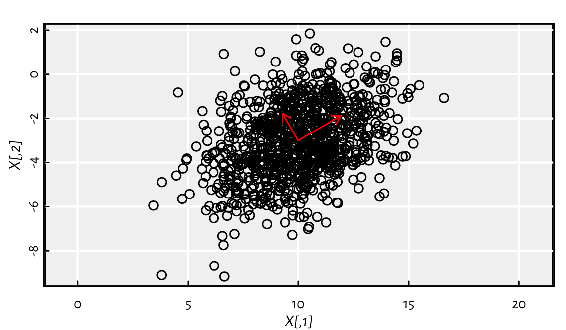
Figure 11.1 A sample from a bivariate normal distribution and its principal axes.
\(\mathbf{X}\) was created by generating a realisation of a two-dimensional standard normal vector \(\mathbf{Z}\), scaling it by \(\left(\sqrt{5}, \sqrt{2}\right)\), rotating by the counterclockwise angle \(\pi/6\), and shifting by \((10, -3)\), which we denote by \(\mathbf{X}=\mathbf{Z} \mathbf{S} \mathbf{R} + \boldsymbol{\mu}^T\). It follows a bivariate[5] normal distribution centred at \(\boldsymbol{\mu}=(10, -3)\) and with the covariance matrix \(\boldsymbol{\Sigma}=(\mathbf{S} \mathbf{R})^T (\mathbf{S} \mathbf{R})\):
crossprod(S %*% R)  # covariance matrix
##       [,1]  [,2]
## [1,] 4.250 1.299
## [2,] 1.299 2.750
cov(X)  # compare: sample covariance matrix (estimator)
##        [,1]   [,2]
## [1,] 4.1965 1.2386
## [2,] 1.2386 2.7973
It is known that eigenvectors of the covariance matrix correspond to the principal components of the original dataset. Furthermore, its eigenvalues give the variances explained by each of them.
eigen(cov(X))
## eigen() decomposition
## $values
## [1] 4.9195 2.0744
##
## $vectors
##          [,1]     [,2]
## [1,] -0.86366  0.50408
## [2,] -0.50408 -0.86366
It roughly corresponds to the principal directions \((\cos \pi/6, \sin \pi/6 )\simeq (0.866, 0.5)\) and the thereto-orthogonal \((-\sin \pi/6, \cos \pi/6 )\simeq (-0.5, 0.866)\) (up to an orientation inverse) with the corresponding variances of 5 and 2, respectively (i.e., standard deviations of \(\sqrt{5}\) and \(\sqrt{2}\)). Note that this method of performing principal component analysis, i.e., recreating the scale and rotation transformation applied on \(\mathbf{Z}\) based only on \(\mathbf{X}\), is not particularly numerically stable; see Exercise 11.26 for an alternative.
11.4.5. QR decomposition
Let \(n\ge m\). We say that a real \(n\times m\) matrix \(\mathbf{Q}\) is orthogonal, whenever \(\mathbf{Q}^T \mathbf{Q} = \mathbf{I}\) (identity matrix). This is equivalent to \(\mathbf{Q}\)’s columns’ being orthogonal unit vectors. Also, if \(\mathbf{Q}\) is a square matrix, then \(\mathbf{Q}^T=\mathbf{Q}^{-1}\) if and only if \(\mathbf{Q}^T \mathbf{Q} = \mathbf{Q} \mathbf{Q}^T = \mathbf{I}\).
Let \(\mathbf{A}\) be a real[6] \(n\times m\) matrix with \(n\ge m\). Then \(\mathbf{A}=\mathbf{Q}\mathbf{R}\) is its QR decomposition, if \(\mathbf{Q}\) is an orthogonal \(n\times m\) matrix and \(\mathbf{R}\) is an upper triangular \(m\times m\) one. Note that such a decomposition is not necessarily unique (without imposing additional requirements), and that we speak here of a QR factorisation in the so-called narrow form.
The qr function returns an object of the S3 class qr
from which we can extract the two components of interest; see the
qr.Q and qr.R functions.
Let \(\mathbf{X}\) be an \(n\times m\) data matrix, representing \(n\) points in \(\mathbb{R}^m\), and a vector \(\mathbf{y}\in\mathbb{R}^n\), where \(y_i\) gives the desired output corresponding to the input \(\mathbf{x}_{i,\cdot}\).
Let \(\boldsymbol\theta\) be a vector of \(m\) parameters. For fitting a linear model \(y=\mathbf{x}^T \boldsymbol\theta=\theta_1 x_1 + \dots+\theta_m x_m\), we can use the method of least squares, which minimises the quadratic loss function:
It might be shown that if we have the QR factorisation \(\mathbf{X}=\mathbf{Q}\mathbf{R}\), then the optimal \(\boldsymbol\theta\) is given by:
which can conveniently be determined via a call to qr.coef.
In particular, we can fit a simple linear regression model \(y=ax+b=\mathbf{x}^T \boldsymbol\theta\) by considering \(\mathbf{x} = (x, 1)\) and \(\boldsymbol\theta = (a, b)\). For instance:
x <- cars[["speed"]]
y <- cars[["dist"]]
X1 <- cbind(x, 1)  # the model is theta[1]*x + theta[2]*1
qrX1 <- qr(X1)
(theta <- qr.coef(qrX1, y))
##        x
##   3.9324 -17.5791
plot(x, y, xlab="speed", ylab="dist")  # scatter plot
abline(theta[2], theta[1], lty=2)  # add the regression line
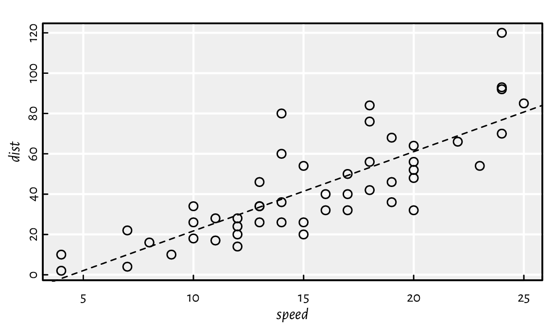
Figure 11.2 The cars dataset and the fitted regression line.
Thus, the fitted model is \(y=3.9324x-17.5791\), see Figure 11.2.
The same approach is used by lm.fit, the workhorse behind the lm method that allows for specifying regression models using an R formula (which some readers might be familiar with; compare Section 17.6).
lm.fit(cbind(x, 1), y)[["coefficients"]]  # also: lm(dist~speed, data=cars)
##        x
##   3.9324 -17.5791
As an exercise, let us compute \(\boldsymbol\theta=\mathbf{R}^{-1}\mathbf{Q}^T\mathbf{y}\) manually. We note that the one-argument version of solve determines the inverse of a given matrix. Thus:
Q <- qr.Q(qrX1)
R <- qr.R(qrX1)
solve(R) %*% t(Q) %*% y  # or solve(R) %*% crossprod(Q, y)
##       [,1]
## x   3.9324
##   -17.5791
However, from the perspective of numerical stability, computing a matrix inverse is rarely a good idea. Multiplying both sides of the equation \(\boldsymbol\theta=\mathbf{R}^{-1}\mathbf{Q}^T\mathbf{y}\) by \(\mathbf{R}\), we get that it holds \(\mathbf{R} \boldsymbol\theta=\mathbf{b}\) with \(\mathbf{b}=\mathbf{Q}^T\mathbf{y}\). This is a triangular system of linear equations, which can be efficiently solved using a designated routine:
backsolve(R, crossprod(Q, y))
##          [,1]
## [1,]   3.9324
## [2,] -17.5791
11.4.6. SVD decomposition
Given a real \(n\times m\) matrix \(\mathbf{X}\), its singular value decomposition (SVD) is given by \(\mathbf{X}=\mathbf{U} \mathbf{D} \mathbf{V}^T\), where \(\mathbf{U}\) and \(\mathbf{V}\) are orthogonal matrices of dimensions \(n\times p\) and \(m\times p\), respectively, and \(\mathbf{D}\) is a \(p\times p\) diagonal matrix with the singular values of \(\mathbf{X}\). It is usually assumed that \(d_{1,1}\ge\dots\ge d_{p,p}\ge 0\), \(p=\min\{n,m\}\), and then the SVD factorisation is unique.
The corresponding svd function may be used to perform the principal component analysis[7]. Namely, if \(\mathbf{X}=\mathbf{U} \mathbf{D} \mathbf{V}^T\), then the columns of \(\mathbf{V}\) give the eigenvectors of \(\mathbf{X}^T \mathbf{X}\). The latter is precisely its scaled covariance matrix if we assume that \(\mathbf{X}\) is centred at \(\boldsymbol{0}\),
(*) Continuing Exercise 11.24 that features a rotated bivariate normal sample, we can determine the principal directions by referring to the \(\mathbf{V}\) component of the SVD decomposition of a centred version of the data matrix:
Xc <- t(t(X)-colMeans(X))  # centred version of X
svd(Xc)[["v"]]
##          [,1]     [,2]
## [1,] -0.86366 -0.50408
## [2,] -0.50408  0.86366
The SVD factorisation can also aid in determining the solution to linear regression. In the previous section, we mentioned that the parameter vector \(\boldsymbol\theta\) minimising \(\|\mathbf{X} \boldsymbol\theta - \mathbf{y}\|_2^2\) is given by \(\boldsymbol\theta = \left(\mathbf{X}^T \mathbf{X} \right)^{-1} \mathbf{X}^T \mathbf{y} \). The component \(\mathbf{X}^+=\left(\mathbf{X}^T \mathbf{X} \right)^{-1} \mathbf{X}^T\) is called the pseudoinverse of \(\mathbf{X}\) for it holds that \(\mathbf{X}^+ \mathbf{X}=\mathbf{I}\). If the SVD decomposition is \(\mathbf{X}=\mathbf{U} \mathbf{D} \mathbf{V}^T\), then \(\mathbf{X}^+=\mathbf{V} \mathbf{D}^+ \mathbf{U}^T\), where \(\mathbf{D}^+\) is the transposed version of \(\mathbf{D}\) carrying the reciprocals of its non-zero elements.
Let us go back to the simple linear regression model discussed in Exercise 11.25. The same solution can be obtained by computing:
svdX1 <- svd(X1)
V <- svdX1[["v"]]
d <- svdX1[["d"]]  # only the elements on the diagonal
U <- svdX1[["u"]]
V %*% diag(1/d) %*% t(U) %*% y
##          [,1]
## [1,]   3.9324
## [2,] -17.5791
The book [8] gives many more applications of the SVD factorisation in data science.
11.4.7. A note on the Matrix package
The Matrix package is perhaps the most widely known showcase of the S4 object orientation (Section 10.5). It defines classes and methods for dense and sparse matrices, including rectangular, symmetric, triangular, band, and diagonal ones. In particular, large graph (e.g., in network sciences) or preference (e.g., in recommender systems) data can be represented using sparse matrices, i.e., those with many zeroes. After all, it is much more likely for two vertices in a network not to be joined by an edge than to be connected. For example:
library("Matrix")
(D <- Diagonal(x=1:5))
## 5 x 5 diagonal matrix of class "ddiMatrix"
##      [,1] [,2] [,3] [,4] [,5]
## [1,]    1    .    .    .    .
## [2,]    .    2    .    .    .
## [3,]    .    .    3    .    .
## [4,]    .    .    .    4    .
## [5,]    .    .    .    .    5
We created a real diagonal matrix of size \(5\times 5\); 20 elements equal to zero are specially marked. Moreover:
S <- as(D, "sparseMatrix")
S[1, 2] <- 7
S[4, 1] <- 42
print(S)
## 5 x 5 sparse Matrix of class "dgCMatrix"
##
## [1,]  1 7 . . .
## [2,]  . 2 . . .
## [3,]  . . 3 . .
## [4,] 42 . . 4 .
## [5,]  . . . . 5
It yielded a general sparse real matrix in the CSC (compressed, sparse, column-orientated) format.
For more information on this package, see
vignette(package="Matrix").
11.5. Exercises
Let X be a matrix with dimnames set. For instance:
X <- matrix(1:12, byrow=TRUE, nrow=3)      # example matrix
dimnames(X)[[2]] <- c("a", "b", "c", "d")  # set column names
print(X)
##      a  b  c  d
## [1,] 1  2  3  4
## [2,] 5  6  7  8
## [3,] 9 10 11 12
Explain the meaning of the following expressions involving matrix subsetting. Note that a few of them are invalid.
X[1, ],X[, 3],X[, 3, drop=FALSE],X[3],X[, "a"],X[,c("a", "b", "c")],X[, -2],X[X[,1] > 5, ],X[X[,1]>5,c("a", "b", "c")],X[X[,1]>=5 & X[,1]<=10, ],X[X[,1]>=5 & X[,1]<=10,c("a", "b", "c")],X[,c(1, "b", "d")].
Assuming that X is an array, what is the difference between the following
operations involving indexing?
X["1", ]vsX[1, ],X[, "a", "b", "c"]vsX["a", "b", "c"]vsX[,c("a", "b", "c")]vsX[c("a", "b", "c")],X[1]vsX[, 1]vsX[1, ],X[X>0]vsX[X>0, ]vsX[, X>0],X[X[, 1]>0]vsX[X[, 1]>0,]vsX[,X[,1]>0],X[X[, 1]>5, X[1, ]<10]vsX[X[1, ]>5, X[, 1]<10].
Give a few ways to create a matrix like:
##      [,1] [,2]
## [1,]    1    1
## [2,]    1    2
## [3,]    1    3
## [4,]    2    1
## [5,]    2    2
## [6,]    2    3
and one like:
##       [,1] [,2] [,3]
##  [1,]    1    1    1
##  [2,]    1    1    2
##  [3,]    1    2    1
##  [4,]    1    2    2
##  [5,]    1    3    1
##  [6,]    1    3    2
##  [7,]    2    1    1
##  [8,]    2    1    2
##  [9,]    2    2    1
## [10,]    2    2    2
## [11,]    2    3    1
## [12,]    2    3    2
For a given real \(n\times m\) matrix \(\mathbf{X}\), encoding \(n\) input points in an \(m\)-dimensional space, determine their bounding hyperrectangle, i.e., return a \(2\times m\) matrix \(\mathbf{B}\) with \(b_{1,j}=\min_i x_{i,j}\) and \(b_{2,j}=\max_i x_{i,j}\).
Let \(\mathbf{t}\) be a vector of \(n\) integers in \(\{1,\dots,k\}\). Write a function to one-hot encode each \(t_i\), i.e., return a 0–1 matrix \(\mathbf{R}\) of size \(n\times k\) such that \(r_{i,j}=1\) if and only if \(j = t_i\) (such a representation is beneficial when solving, e.g., a multiclass classification problem by means of \(k\) binary classifiers). For example, if \(\mathbf{t}=[1, 2, 3, 2, 4]\) and \(k=4\), then:
Then, compose another function, but this time setting \(r_{i,j}=1\) if and only if \(j\ge t_i\), e.g.:
Important
As usual, try to solve all the exercises without using explicit for and while loops (provided that it is possible).
Given an \(n\times k\) real matrix, apply the softmax function on each row, i.e., map \(x_{i,j}\) to \(\frac{\exp(x_{i,j})}{\sum_{l=1}^k \exp(x_{i,l})}\). Then, one-hot decode the values in each row, i.e., find the column number with the greatest value. Return a vector of size \(n\) with elements in \(\{1,\dots,k\}\).
Assume that an \(n\times m\) real matrix \(\mathbf{X}\) represents \(n\) points in \(\mathbb{R}^m\). Write a function (but do not refer to dist) that determines the pairwise Euclidean distances between all the \(n\) points and a given \(\mathbf{y}\in\mathbb{R}^m\). Return a vector \(\mathbf{d}\) of length \(n\) with \(d_{i}=\|\mathbf{x}_{i,\cdot}-\mathbf{y}\|_2\).
Let \(\mathbf{X}\) and \(\mathbf{Y}\) be two real-valued matrices of sizes \(n\times m\) and \(k\times m\), respectively, representing two sets of points in \(\mathbb{R}^m\). Return an integer vector \(\mathbf{r}\) of length \(k\) such that \(r_i\) indicates the index of the point in \(\mathbf{X}\) with the least distance to (the closest to) the \(i\)-th point in \(\mathbf{Y}\), i.e., \(r_i = \mathrm{arg}\min_j \|\mathbf{x}_{j,\cdot}-\mathbf{y}_{i,\cdot}\|_2\).
Write your version of utils::combn.
Time series are vectors or matrices of the class ts
equipped with the tsp attribute, amongst others.
Refer to help("ts") for more information about
how they are represented and what S3 methods have been overloaded for them.
(*) Numeric matrices can be stored in a CSV file, amongst others. Usually, we will be loading them via read.csv, which returns a data frame (see Chapter 12). For example:
X <- as.matrix(read.csv(
    paste0(
        "https://github.com/gagolews/teaching-data/",
        "raw/master/marek/eurxxx-20200101-20200630.csv"
    ),
    comment.char="#",
    sep=","
))
Write a function
read_numeric_matrix(file_name, comment, sep)
which is based on a few calls to scan instead.
Use file to establish a file connection so that you can
ignore the comment lines and fetch the column names
before reading the actual numeric values.
(*)
Using readBin, read the t10k-images-idx3-ubyte.gz from the
MNIST database homepage.
The output object should be a three-dimensional, \(10000\times 28\times 28\)
array with real elements between 0 and 255. Refer to the File Formats
section therein for more details.
(**) Circular convolution of discrete-valued multidimensional signals can be performed by means of fft and matrix multiplication, whereas affine transformations require only the latter. Apply various image transformations such as sharpening, shearing, and rotating on the MNIST digits and plot the results using the image function.
(*) Using constrOptim, find the minimum of the Constrained Betts Function \(f(x_1, x_2) = 0.01 x_1^2 + x_2^2 - 100\) with linear constraints \( 2\le x_1 \le 50\), \(-50 \le x_2 \le 50\), and \(10 x_1 \ge 10 + x_2\). (**) Also, use solve.QP from the quadprog package to find the minimum.