17. Lazy evaluation (**)

This open-access textbook is, and will remain, freely available for everyone’s enjoyment (also in PDF; a paper copy can also be ordered). It is a non-profit project. Although available online, it is a whole course, and should be read from the beginning to the end. Refer to the Preface for general introductory remarks. Any bug/typo reports/fixes are appreciated. Make sure to check out Minimalist Data Wrangling with Python [27] too.

The ability to create, store, and manipulate unevaluated expressions so that they can be computed later is not particularly special. Many languages enjoy such metaprogramming (computing on the language, reflection) capabilities, e.g., Lisp, Scheme, Wolfram, Julia, amongst many others.

However, R inherited from its predecessor, the S language, a variation of lazy[1] (nonstrict, noneager, delayed) evaluation of function arguments. They are only computed when their values are first needed. As we can take the expressions used to generate them (via substitute; see Section 15.4.2), we shall see that we can ignore their meaning in the original (caller’s) context and compute them in a very different one.

17.1. Evaluation of function arguments

We know that calls such as `if`(test, ifyes, ifno), `||`(mustbe, maybe), or `&&`(mustbe, maybe) do not have to evaluate all their arguments.

{cat(" first "); FALSE} && {cat(" second "); FALSE}
##  first
## [1] FALSE
{cat(" first "); TRUE } && {cat(" Spanish Inquisition "); FALSE}
##  first  Spanish Inquisition
## [1] FALSE

We can compose such functions ourselves. For instance:

test <- function(a, b, c) a + c  # b is unused
test({cat("spam\n"); 1}, {cat("eggs\n"); 10}, {cat("salt\n"); 100})
## spam
## salt
## [1] 101

The second argument was not referred to in the function’s body. Therefore, it was not evaluated (no printing of eggs occurred).

Example 17.1

Study the following very carefully.

test <- function(a, b, c)
{
    cat("Arguments passed to `test` (expressions): \n")
    cat("a = ", deparse(substitute(a)), "\n")
    cat("b = ", deparse(substitute(b)), "\n")
    cat("c = ", deparse(substitute(c)), "\n")

    subtest <- function(x, y, z)
    {
        cat("Arguments passed to `subtest` (expressions): \n")
        cat("x = ", deparse(substitute(x)), "\n")
        cat("y = ", deparse(substitute(y)), "\n")
        cat("z = ", deparse(substitute(z)), "\n")
        cat("Using x and z... ")
        retval <- x + z  # does not refer to `y`
        cat("Cheers!\n")
        retval
    }

    cat("Using c... ")
    c  # force evaluation; we do not even have to be particularly creative

    subtest(a, ~!~b*2 := headache ->> ha@x$y, c*10)  # no evaluation yet!
}

environment(test) <- new.env()  # to spice things up

test(
    {testx <- "goulash"; cat("spam\n"); 1},
    {testy <- "kabanos"; cat("eggs\n"); MeAn(egGs+whatever&!!weird[stuff])},
    {testx <- "kransky"; cat("salt\n"); 100}
)
## Arguments passed to `test` (expressions):
## a =  {     testx <- "goulash"     cat("spam\n")     1 }
## b =  {     testy <- "kabanos"     cat("eggs\n")     MeAn(egGs + whatever …
## c =  {     testx <- "kransky"     cat("salt\n")     100 }
## Using c... salt
## Arguments passed to `subtest` (expressions):
## x =  a
## y =  `:=`(~!~b * 2, ha@x$y <<- headache)
## z =  c * 10
## Using x and z... spam
## Cheers!
## [1] 1001
print(testx)
## [1] "goulash"
print(testy)
## Error in eval(expr, envir, enclos): object 'testy' not found

On a side note, the `~` (formula) operator will be discussed in Section 17.6. Furthermore, the `:=` operator was used in an ancient version of R for assignments. The parser still recognises it, yet now it has no associated meaning.

Important

We note what follows.

• Either the evaluation of an argument does not happen, or is triggered only once (in which case the result is cached).

  This is why, in our example, salt was printed once.

• Evaluation is delayed until the very first request for the underlying value. We call it lazy evaluation.

  It can be delayed forever; eggs is never printed and testy is undefined.

• Evaluation takes place in the calling environment (parent frame).

  testx is equal to goulash after all.

• Merely passing arguments further to another function usually does not trigger the evaluation.

  We wrote usually because functions of the type builtin (e.g., c, list, sum, `+`, `&`, and `:`) always evaluate the arguments. There is no lazy evaluation in the case of the arguments passed to group generics; see help("groupGeneric") and Section 10.2.6. Furthermore, replacement functions’ values arguments (Section 9.3.6) are computed eagerly.

• Fetching the expression passed as an argument using substitute (Section 15.4.2) or checking if an argument was provided with missing (Section 15.4.3) does not trigger the evaluation.

  We see spam printed much later.

Exercise 17.2

Study the source code of system.time and notice the use of delayed evaluation to measure the duration of the execution of a given expression. Note that on.exit (Section 17.4) reacts to possible exceptions.

Example 17.3

It turns out that the role of substitute is broader than just getting the expression passed as an argument. We can actually replace each occurrence of every name from a given dictionary (a named list or an environment). For instance:

test <- function(x)
{
    subtest <- function(y)
    {
        ex <- substitute(x, env=parent.frame())  # substitute(x) is just `x`
        ey <- substitute(y)
        cat("ex =", deparse(ex), "\n")
        cat("ey =", deparse(ey), "\n")
        # not: eval(substitute(ey, list(x=ex)))
        eval(as.call(list(substitute, ey, list(x=ex))))
    }

    subtest(spam(!x[x](x)))
}

test(eels@hovercraft)
## ex = eels@hovercraft
## ey = spam(!x[x](x))
## spam(!eels@hovercraft[eels@hovercraft](eels@hovercraft))

We fetched the expression passed as the x argument to the calling function. Then, we replaced every occurrence of x in the expression ey. On a side note, as substitute does not evaluate its first argument, if we called substitute(ey, ...) in the last expression of subtest, we would treat ey as a quoted name.

Exercise 17.4

Study the source code of replicate:

print(replicate)
## function (n, expr, simplify = "array")
## sapply(integer(n), eval.parent(substitute(function(...) expr)),
##     simplify = simplify)
## <environment: namespace:base>

It creates a function that evaluates expr inside its local environment, which is new every time. Note that eval.parent(expr) is a shorthand for eval(expr, parent.frame()).

Note

(*) Internally, lazy evaluation of arguments is implemented using the so-called promises, compare [69], which consist of:

• an expression (which we can access by calling substitute);

• an environment where the expression is to be evaluated (once this happens, it is set to NULL);

• a cached value (computed on demand, once).

This interface is not really visible from within R, but see help("delayedAssign").

Exercise 17.5

Inspect the definition of match.fun. Why is it called by, e.g., apply, Map, or outer? Note that it uses eval.parent(substitute(substitute(FUN))) to fetch the expression representing the argument passed by the calling function (but it is probably very rarely needed there). Compare:

test <- function(x)
{
    subtest <- function(y)
    {
        # NOT: substitute(y)
        # NOT: eval.parent(substitute(y))
        eval.parent(substitute(substitute(y)))
    }

    subtest(x*3)
}

test(1+2)
## (1 + 2) * 3

Exercise 17.6

(*) Implement your version of the bquote function.

17.2. Evaluation of default arguments

As we know from Section 9.4.4, default arguments are special expressions specified in a function’s parameter list.

Important

When a function’s body requires the value of an argument that the caller did not provide, the default expression will be evaluated in the current (local) environment of the function.

It is thus different from the case of normally passed arguments, which are interpreted in the context of the calling environment.

Example 17.7

Study the following very carefully.

x <- "banana"

test <- function(y={cat("spam\n"); x})
{
    cat(deparse(substitute(y)), "\n")
    cat("bacon\n")
    x <- "rotten potatoes"
    cat(y, y, "\n")
}

test({cat("spam\n"); x})
## {     cat("spam\n")     x }
## bacon
## spam
## banana banana

As usual, the evaluation is triggered only once, where it was explicitly requested, and only when needed. y was bound to the value of x from the calling environment (banana in the global one).

test()
## {     cat("spam\n")     x }
## bacon
## spam
## rotten potatoes rotten potatoes

The expression for the default y was evaluated in the local environment. It happened after the creation of the local x.

Example 17.8

Consider the following example from [37]:

sumsq <- function(y, about=mean(y), na.rm=FALSE)
{
    if (na.rm)
        y <- y[!is.na(y)]
    sum((y - about)^2)
}

y <- c(1, NA_real_, NA_real_, 2)
sumsq(y, na.rm=TRUE)
## [1] 0.5

In the case where we rely on the default argument, the computation of the mean may take into account the request for missing value removal. Still, the following will not work as intended:

sumsq(y, mean(y), na.rm=TRUE)  # we should rather pass mean(y, na.rm=TRUE)
## [1] NA

However, as the idea of lazy evaluation of arguments is alien to most programmers (especially those coming from different languages), it might be better to rewrite the above using a call to missing (Section 15.4.3):

sumsq <- function(y, about, na.rm=FALSE)
{
    if (na.rm)
        y <- y[!is.na(y)]
    if (missing(about))
        about <- mean(y)
    sum((y - about)^2)
}

sumsq(y, na.rm=TRUE)
## [1] 0.5

or better even:

sumsq <- function(y, about=NULL, na.rm=FALSE)
{
    if (na.rm)
        y <- y[!is.na(y)]
    if (is.null(about))
        about <- mean
    sum((y - about(y))^2)
}

sumsq(y, na.rm=TRUE)
## [1] 0.5

Exercise 17.9

The default arguments to do.call, list2env, and new.env are set to parent.frame. What does that mean?

Exercise 17.10

Study the source code of the local function:

print(local)
## function (expr, envir = new.env())
## eval.parent(substitute(eval(quote(expr), envir)))
## <environment: namespace:base>

17.3. Ellipsis revisited

If our function has the dot-dot-dot parameter, `...`, whatever we pass through it is packed into a pairlist of promise expressions. Thus, we can relish the benefits of lazy evaluation. In particular, we can redirect all `...`-fed arguments to another call as-is.

test <- function(...)
{
    subtest <- function(x, ...)
    {
        cat("x   = "); str(x)
        cat("... = "); str(list(...))
    }

    subtest(...)
}

test({cat("eggs! "); 1}, {cat("spam! "); 2}, z={cat("rice! "); 3})
## x   = eggs!  num 1
## ... = spam! rice! List of 2
##  $  : num 2
##  $ z: num 3

Exercise 17.11

In the documentation of lapply, we read that this function is called like lapply(X, FUN, ...), where `...` are optional arguments to FUN. Verify that whatever is passed via the ellipsis is evaluated only once and not on each application of FUN on the elements of X.

Example 17.12

We know from Chapter 13 that many high-level graphics functions rely on multiple calls to more primitive routines that allow for setting a variety of parameters (e.g., via par). A common scenario is for a high-level function to pass all the arguments down. Each underlying procedure can then decide by itself which items it is interested in.

test <- function(...)
{
    subtest1 <- function(..., a=1) c(a=a)
    subtest2 <- function(..., b=2) c(b=b)
    subtest3 <- function(..., c=3) c(c=c)

    c(subtest1(...), subtest2(...), subtest3(...))
}

test(a="A", b="B", d="D")
##   a   b   c
## "A" "B" "3"

Here, for instance, subtest1 only consumes the value of a and ignores all other arguments whatsoever. plot.default (amongst others) relies on such a design pattern.

`...length` fetches the number of items passed via the ellipsis, `...names` retrieves their names (in the case they are given as keyword arguments), and `...elt`(i) gives the value of the \(i\)-th element. Furthermore, `..1`, `..2`, and so forth are synonymous with `...elt`(1), `...elt`(2), etc.

test <- function(...)
{
    cat("length:", ...length(), "\n")
    cat("names: ", paste(...names(), collapse=", "), "\n")
    for (i in seq_len(...length()))
        cat(i, ":", ...elt(i), "\n")
    print(substitute(...elt(i)))
}

test(u={cat("honey! "); "a"}, {cat("gravy! "); "b"}, w={cat("bacon! "); "c"})
## length: 3
## names:  u, , w
## honey! 1 : a
## gravy! 2 : b
## bacon! 3 : c
## ...elt(3L)

Note that `...elt`(i) triggers the evaluation of the respective argument. Unfortunately, we cannot use substitute to fetch the underlying expression. Instead, we can rely on match.call discussed in Section 15.4.4:

test <- function(a, b, ..., z=1)
{
    e <- match.call()[-1]
    as.list(e[!(names(e) %in% names(formals(sys.function())))])
}

str(test(1+1, 2+2, 3+3, 4+4, a=2, z=8, w=4))
## List of 4
##  $  : language 2 + 2
##  $  : language 3 + 3
##  $  : language 4 + 4
##  $ w: num 4

Note

Objects passed via `...`, even if they are specified as keyword arguments, cannot be referred to by their name as if they were local variables:

test <- function(...) zzz
test(zzz=3)
## Error in test(zzz = 3): object 'zzz' not found

In other words, no assignment in the local environment is triggered.

Exercise 17.13

Implement your version of the switch function.

Exercise 17.14

Write your version of the stopifnot function.

17.4. on.exit (*)

on.exit registers an expression to be evaluated at the very end of a call, regardless of whether the function exited due to an error or not. It might be used to reset the temporarily modified graphics parameters (see par) and system options (options) or clean up the allocated resources (e.g., close all open file connections). For instance:

test <- function(reset=FALSE, error=FALSE)
{
    on.exit(cat("eggs\n"))
    on.exit(cat("bacon\n"))  # replace
    on.exit(cat("spam\n"), add=TRUE)  # add

    cat("roti canai\n")

    if (reset)
        on.exit()  # cancels all (replace by nothing)

    if (error)
        stop("aaarrgh!")

    cat("end\n")
    "return value"
}

test()
## roti canai
## end
## bacon
## spam
## [1] "return value"
test(reset=TRUE)
## roti canai
## end
## [1] "return value"
test(error=TRUE)
## roti canai
## Error in test(error = TRUE): aaarrgh!
## bacon
## spam

We can always manage without on.exit, e.g., by applying exception handling techniques; see Section 8.2.

Exercise 17.15

In the definition of scan, notice the call to:

on.exit(close(file))

Is its purpose to close the file on exit?

Exercise 17.16

Why does graphics::barplot.default call the following expressions?

dev.hold()
opar <- if (horiz) par(xaxs="i", xpd=xpd) else par(yaxs="i", xpd=xpd)
on.exit({
    dev.flush()
    par(opar)
})

17.5. Metaprogramming and laziness in action: Examples (*)

Due to lazy evaluation, we can define functions that permit any random syntactically valid gibberish to be fed as their arguments. Nothing but basic decency stops us from interpreting them in any way we want. Each such function can become a microverse (a microlanguage?) by itself. This will surely confuse[2] our users, as they will have to analyse every procedure’s behaviour separately.

In this section, we extend on our notes from Section 9.4.7 and Section 12.3.9. We look at a few functions relying on metaprogramming and laziness, mostly because studying them is a good exercise. It can help extend our programming skills and deepen our understanding of the concepts discussed in this part of the book. By no means is it an invitation to use them in practice. Nevertheless, R’s computing on the language capabilities might interest some advanced programmers (e.g., package developers).

17.5.1. match.arg

match.arg was mentioned in Section 9.4.7. When called normally, it matches a string against a set of possible choices, similarly to pmatch:

choices <- c("spam", "bacon", "eggs")
match.arg("spam", choices)
## [1] "spam"
match.arg("s", choices)  # partial matching
## [1] "spam"
match.arg("eggplant", choices)  # no match
## Error in match.arg("eggplant", choices): 'arg' should be one of "spam",
##     "bacon", "eggs"
match.arg(choices, choices)  # match first
## [1] "spam"

However, skipping the second argument, this function will fetch the choices from the default argument of the function it is enclosed in!

test <- function(x=c("spam", "bacon", "eggs"))
    match.arg(x)

test("spam")
## [1] "spam"
test("s")
## [1] "spam"
test("eggplant")
## Error in match.arg(x): 'arg' should be one of "spam", "bacon", "eggs"
test()
## [1] "spam"

Exercise 17.17

Inspect the source code of stats::binom.test, which looks like:

function(..., alternative = c("two.sided", "less", "greater"))
{
    # ...
    alternative <- match.arg(alternative)
    # ...
}

Read the description of the alternative argument in the documentation.

Exercise 17.18

Study the source code of match.arg. In particular, notice the following fragment:

if (missing(choices)) {
    formal.args <- formals(sys.function(sysP <- sys.parent()))
    choices <- eval(
        formal.args[[as.character(substitute(arg))]],
        envir=sys.frame(sysP)
    )
}

17.5.2. curve

The curve function can be called, e.g., like:

curve(sin(1/x^2), 1/pi, 3, 1001, lty=2)

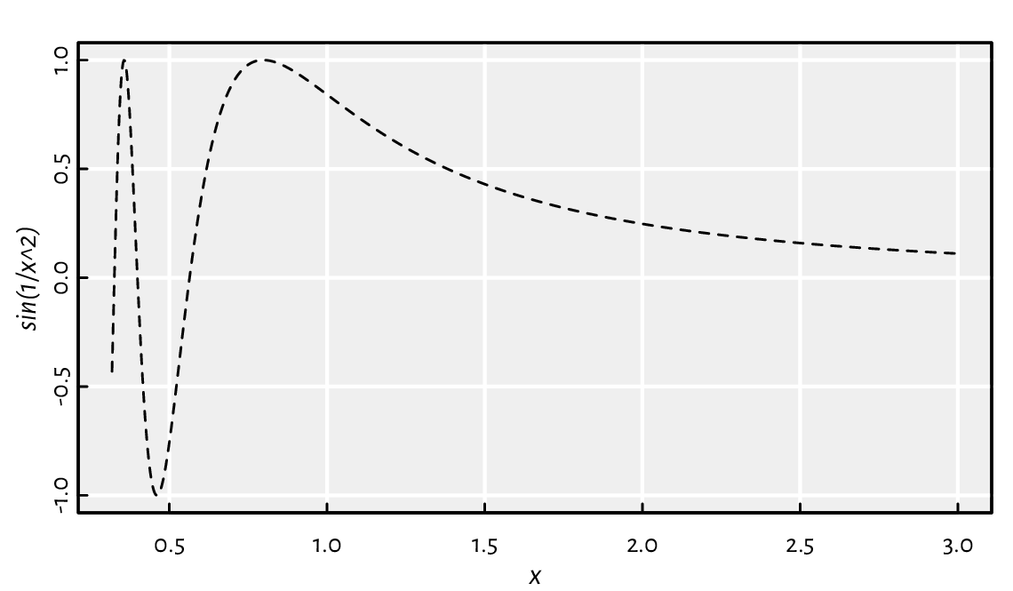
Figure 17.1 An example plot generated by calling curve.

It results in Figure 17.1. Wait a minute… We did not define x as a sequence ranging between about 0.3 and 3!

Exercise 17.19

Study the source code of curve. Take note of the following code fragment:

function(expr, from=NULL, to=NULL, n=101, xlab="x", type="l", ...)
{
    # ...
    expr <- substitute(expr)
    ylab <- deparse(expr)
    x <- seq.int(from, to, length.out=n)
    ll <- list(x=x)
    y <- eval(expr, envir=ll, enclos=parent.frame())
    plot(x=x, y=y, type=type, xlab=xlab, ylab=ylab, ...)
    # ...
}

17.5.3. with and within

Environments and named lists (and hence data frames) are similar (Section 16.1.2). Due to this, the envir argument to eval can be set to either. Therefore, for instance:

eval(quote(head(Sepal.Length)), envir=iris)
## [1] 5.1 4.9 4.7 4.6 5.0 5.4

It evaluates the given expression in something like list2env(iris, parent=parent.frame()). Thus, even though Sepal.Length is not a standalone variable, it is treated as one inside the iris data frame.

Moreover, the enclosure is set to the calling frame. Hence, we can successfully refer to the head function located somewhere on the search path. This is somewhat similar to attach (Section 16.2.6) but without modifying the search path.

The with function does exactly the above:

print(with.default)
## function (data, expr, ...)
## eval(substitute(expr), data, enclos = parent.frame())
## <environment: namespace:base>

Example use:

with(iris, {
    mean(Sepal.Length)  # `Sepal.Length` is in `iris`
})
## [1] 5.8433

As we evaluate it in the local (temporary) environment, we cannot modify the existing columns of the data frame this way. However, the within function includes a way to detect and apply any changes made.

within(iris, {
    Sepal.Length <- Sepal.Length/1000
    Spam <- "yum!"
}) -> iris2
head(iris2, 3)
##   Sepal.Length Sepal.Width Petal.Length Petal.Width Species Spam
## 1       0.0051         3.5          1.4         0.2  setosa yum!
## 2       0.0049         3.0          1.4         0.2  setosa yum!
## 3       0.0047         3.2          1.3         0.2  setosa yum!

Exercise 17.20

Study the source code of within:

print(within.data.frame)
## function (data, expr, ...)
## {
##     parent <- parent.frame()
##     e <- evalq(environment(), data, parent)
##     eval(substitute(expr), e)
##     l <- as.list(e, all.names = TRUE)
##     l <- l[!vapply(l, is.null, NA, USE.NAMES = FALSE)]
##     nl <- names(l)
##     del <- setdiff(names(data), nl)
##     data[nl] <- l
##     data[del] <- NULL
##     data
## }
## <environment: namespace:base>

Note that evalq(expr, ...) is equivalent to eval(quote(expr), ...). Also, vapply(X, FUN, NA, ...) is like a call to sapply, but it guarantees that the result is a logical vector.

17.5.4. transform

We can call transform to modify/add columns in a data frame using vectorised functions. For instance:

head(transform(mtcars, log_hp=log(hp), am=2*am-1, hp=NULL), 3)
##                mpg cyl disp drat    wt  qsec vs am gear carb log_hp
## Mazda RX4     21.0   6  160 3.90 2.620 16.46  0  1    4    4 4.7005
## Mazda RX4 Wag 21.0   6  160 3.90 2.875 17.02  0  1    4    4 4.7005
## Datsun 710    22.8   4  108 3.85 2.320 18.61  1  1    4    1 4.5326

If we suspect that this function evaluates all expressions passed as `...` within the data frame, we are brilliantly right. Furthermore, there must be a mechanism to detect newly created variables so that new columns can be added.

Exercise 17.21

Study the source code of transform:

print(transform.data.frame)
## function (`_data`, ...)
## {
##     e <- eval(substitute(list(...)), `_data`, parent.frame())
##     tags <- names(e)
##     inx <- match(tags, names(`_data`))
##     matched <- !is.na(inx)
##     if (any(matched)) {
##         `_data`[inx[matched]] <- e[matched]
##         `_data` <- data.frame(`_data`)
##     }
##     if (!all(matched))
##         do.call("data.frame", c(list(`_data`), e[!matched]))
##     else `_data`
## }
## <environment: namespace:base>

In particular, note that e is a named list.

17.5.5. subset

The subset function selects rows and columns of a data frame that meet certain criteria. For instance:

subset(airquality, Temp>95 | Temp<57, -(Month:Day))
##     Ozone Solar.R Wind Temp
## 5      NA      NA 14.3   56
## 120    76     203  9.7   97
## 122    84     237  6.3   96

The second argument, the row selector, must definitely be evaluated within the data frame. We expect it to reduce itself to a logical vector which can then be passed to the index operator.

The “select all columns except those between the given ones” part can be implemented by assigning each column a consecutive integer and then treating them as numeric indexes.

Exercise 17.22

Study the source code of subset:

print(subset.data.frame)
## function (x, subset, select, drop = FALSE, ...)
## {
##     chkDots(...)
##     r <- if (missing(subset))
##         rep_len(TRUE, nrow(x))
##     else {
##         e <- substitute(subset)
##         r <- eval(e, x, parent.frame())
##         if (!is.logical(r))
##             stop("'subset' must be logical")
##         r & !is.na(r)
##     }
##     vars <- if (missing(select))
##         rep_len(TRUE, ncol(x))
##     else {
##         nl <- as.list(seq_along(x))
##         names(nl) <- names(x)
##         eval(substitute(select), nl, parent.frame())
##     }
##     x[r, vars, drop = drop]
## }
## <environment: namespace:base>

17.5.6. Forward pipe operator

Section 10.4 mentioned the pipe operator, `|>`. We can compose its simplified version manually:

`%>%` <- function(e1, e2)
{
    e2 <- as.list(substitute(e2))
    e2 <- as.call(c(e2[[1]], substitute(e1), e2[-1]))
    eval(e2, envir=parent.frame())
}

This function imputes e1 as the first argument in a call e2 and then evaluates the new expression.

Example calls:

x <- c(1, NA_real_, 2, 3, NA_real_, 5)
x %>% mean  # mean(x)
## [1] NA
x %>% `-`(1)  # x-1
## [1]  0 NA  1  2 NA  4
x %>% na.omit %>% mean  # mean(na.omit(x))
## [1] 2.75
x %>% mean(na.rm=TRUE)  # mean(x, na.rm=TRUE)
## [1] 2.75

Moreover, we can memorise the value of e1 so that it can be referred to in the expression on the right side of the operator. This comes at a cost of forcing the evaluation of the left-hand side argument and thus losing the potential benefits of laziness, including access to the generating expression.

`%.>%` <- function(e1, e2)
{
    env <- list2env(list(.=e1), parent=parent.frame())
    e2 <- as.list(substitute(e2))
    e2 <- as.call(c(e2[[1]], quote(.), e2[-1]))
    eval(e2, envir=env)
}

This way, we can refer to the value of the left side multiple times in a single call. For instance:

runif(5) %.>% `[`(.>0.5)   # x[x>0.5] with x=runif(5)
## [1] 0.78831 0.88302 0.94047

This is crazy, I know. I made this. Your author. One more then:

# x[x >= 0.5 & x <= 0.9] <- NA_real_ with x=round(runif(5), 2):
runif(5) %.>% round(2) %.>% `[<-`(.>=0.5 & .<=0.9, value=NA_real_)
## [1] 0.29   NA 0.41   NA 0.94

I cannot wait for someone to put this operator into a new R package (it is a brilliant idea, by the way, isn’t it?) and then confuse thousands of users (“What is this thing?”).

17.5.7. Other ideas (**)

Why stop ourselves here? We can create way more invasive functions that read the local variables in the calling functions (unless they are primitive; in R, there are often exceptions to general rules…). Here is an operator which helps select a range of columns in a data frame between two given labels:

`%:%` <- function(e1, e2)
{
    # get the `x` argument in the caller (hoping its `[`)
    x <- get("x", envir=sys.frame(sys.nframe()-1))
    n <- names(x)
    from <- pmatch(substitute(e1), n)
    to <- pmatch(substitute(e2), n)
    from:to
}

head(iris[, Sepal.W%:%Petal.W])
##   Sepal.Width Petal.Length Petal.Width
## 1         3.5          1.4         0.2
## 2         3.0          1.4         0.2
## 3         3.2          1.3         0.2
## 4         3.1          1.5         0.2
## 5         3.6          1.4         0.2
## 6         3.9          1.7         0.4

This operator relies on the assumption that it is called in the expression passed as an argument to a non-primitive function which also takes a named vector x as an actual parameter. So ugly, but saves a few keystrokes. We will not be using it because it is not good for us.

Exercise 17.23

Make the foregoing more foolproof:

• if `%:%` is used outside of `[` or `[<-`, raise a polite error,

• permit x to be a matrix (is it possible?),

• prepare better for the case of less expected inputs.

Exercise 17.24

Modify the definition of the aforementioned operator so that both:

iris[, -Sepal.W%:%Petal.W]
iris[, -(Sepal.W%:%Petal.W)]

mean “select everything except”.

Exercise 17.25

Define `%:%` for data frames so that:

• x[%:%3, ] means “select the first three rows”,

• x[3%:%, ] means “select from the third to the end”,

• x[-3%:%, ] means “select from the third last to the end”,

• x[%:%-10, ] means “select all but the last nine”.

You can go one step further and redefine `[` entirely to support such kinds of indexers.

The ceiling is the limit. Please, do not use it in production.

17.6. Processing formulae, `~` (*)

Formulae were introduced to S in the early 1990s [13]. Their original raison d’être was to specify statistical models; compare Section 10.3.4.

From the language perspective, they are merely unevaluated calls to the `~` (tilde) operator. When creating them, we do not even have to apply quote explicitly. For instance:

f <- (y ~ x1 + x2)  # or: `~`(y, x1+x2)
mode(f)
## [1] "call"
class(f)
## [1] "formula"

Hence, formulae are compound objects in the sense given in Chapter 10. Usually, they are equipped with an additional attribute:

attr(f, ".Environment")  # environment active when the formula was created
## <environment: R_GlobalEnv>

Exercise 17.26

Write a function that generates a list of formulae of the form “y ~ x1+x2+...+xk”, for all possible combinations x1, x2, …, xk (of any cardinality) of elements in a given set of xs. For instance:

formula_allcomb <- function(y, xs, env=parent.frame()) ...to.do...
str(formula_allcomb("len", c("supp", "dose")))
## List of 3
##  $ :Class 'formula'  language len ~ supp + dose
##   .. ..- attr(*, ".Environment")=<environment: R_GlobalEnv>
##  $ :Class 'formula'  language len ~ dose
##   .. ..- attr(*, ".Environment")=<environment: R_GlobalEnv>
##  $ :Class 'formula'  language len ~ supp
##   .. ..- attr(*, ".Environment")=<environment: R_GlobalEnv>
str(formula_allcomb(
    "y",
    c("x1", "x2", "x3"),
    env=NULL
))
## List of 7
##  $ :Class 'formula'  language y ~ x1 + x2 + x3
##  $ :Class 'formula'  language y ~ x2 + x3
##  $ :Class 'formula'  language y ~ x1 + x3
##  $ :Class 'formula'  language y ~ x3
##  $ :Class 'formula'  language y ~ x1 + x2
##  $ :Class 'formula'  language y ~ x2
##  $ :Class 'formula'  language y ~ x1

As they are unevaluated calls, functions can assign any fantastic meaning to formulae. We cannot really do anything about this freedom of expression. However, many functions, especially in the stats and graphics packages, rely on a call to model.frame and related routines. Thanks to this, we can at least find a few behavioural patterns. In particular, help("formula") lists the typical meanings of operators that can be used in a formula.

Example 17.27

Here are a few examples (executing these expressions is left as an exercise).

• Draw a box-and-whisker plot for iris[["Sepal.Length"]] split by iris[["Species"]]:

  boxplot(Sepal.Length~Species, data=iris)
  

• Draw a box plot for ToothGrowth[["len"]] split by a combination of levels in ToothGrowth[["supp"]] and ToothGrowth[["dose"]]:

  boxplot(len~supp:dose, data=ToothGrowth)
  

• Split the given data frame by a combination of values in two specified columns therein:

  split(ToothGrowth, ~supp:dose)
  

• Fit a linear regression model of the form \(y=a+bx\), where \(y\) is iris[["Sepal.Length"]] and \(x\) is iris[["Petal.Length"]]:

  lm(Sepal.Length~Petal.Length, data=iris)
  

• Fit a linear regression model without the intercept term of the form \(z=ax+by\), where \(z\) is iris[["Sepal.Length"]], \(x\) is iris[["Petal.Length"]], and \(y\) is iris[["Sepal.Width"]]:

  lm(Sepal.Length~Petal.Length+Sepal.Width+0, data=iris)
  

• Fit a linear regression model of the form \(z=a+bx+cy+dxy\), where \(z\) is iris[["Sepal.Length"]]+e (with e fetched from the associated environment), and \(x\) and \(y\) are like above:

  e <- rnorm(length(iris[["Sepal.Length"]]), 0, 0.05)
  lm(I(Sepal.Length+e)~Petal.Length*Sepal.Width, data=iris)
  

• Draw scatter plots of warpbreaks[["breaks"]] vs their indexes for data grouped by a combination of warpbreaks[["wool"]] and warpbreaks[["tension"]]:

  Index <- seq_len(NROW(warpbreaks))
  coplot(breaks ~ Index | wool * tension, data=warpbreaks)
  

From the perspective of this book, which focuses on more universal aspects of the R language, formulae are not interesting enough to describe them in any more detail. However, the tender-hearted reader is now equipped with all the necessary knowledge to solve the following very educative exercises.

Exercise 17.28

Study the source code of graphics:::boxplot.formula, stats::lm, and stats:::t.test.formula and notice how they prepare and process the calls to model.frame, model.matrix, model.response, model.weights, etc. Note that their main aim is to prepare data to be passed to boxplot.default, lm.fit (it is just a function with such a name, not an S3 method), and t.test.default.

Exercise 17.29

Write a function similar to curve, but one that lets us specify the function to plot using a formula.

17.7. Exercises

Exercise 17.30

Answer the following questions.

• What is the role of promises?

• Why do we generally discourage the use of functions relying on metaprogramming?

• How are default arguments evaluated?

• Is there anything special about formulae from the language perspective?

• R evaluates function arguments lazily. Does it mean that “y[c(length(y)+1, length(y)+1, length(y)+1)] <- list(1, 2, 3)” extends a list y by three elements? Or are there cases where evaluation is eager?

Exercise 17.31

Why the two following calls yield different results?

test <- function(x, y=deparse(substitute(x)), force_first=FALSE)
{
    if (force_first) y  # just force the evaluation of `y` here
    x <- x**2
    print(y)
}

test(1:5)
## [1] "c(1, 4, 9, 16, 25)"
test(1:5, force_first=TRUE)
## [1] "1:5"

17.8. Outro

Recall our first approximation to the classification of R data types that we presented in the Preface. To summarise what we have covered in this book, let’s contemplate Figure 17.2, which gives a much broader picture.

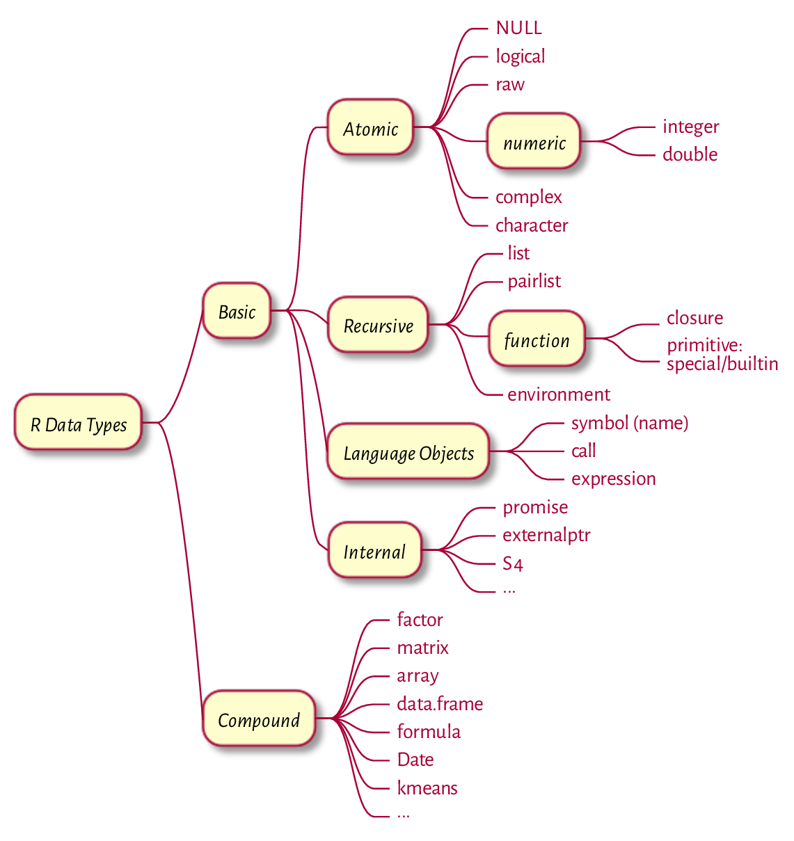
Figure 17.2 R data types.

If we omitted something, it was most likely on purpose: either we can now study it on our own easily, it is not really worth our attention, or it violates our minimalist design principles that we explained in the Preface.

Now that we have reached the end of this course, we might be interested in reading:

• R Language Definition [69],

• R Internals [68],

• Writing R Extensions [65],

• R’s source code available at https://cran.r-project.org/src/base.

What is more, the NEWS files available at https://cran.r-project.org/doc/manuals/r-release will keep us updated with fresh features, bug fixes, and newly deprecated functionality; see also the news function.

Please spread the news about this book. Also, check out another open-access work by yours truly, Minimalist Data Wrangling with Python [27]. Thank you.

Good luck with your further projects!

---

[1]

Call-by-need but without the memoisation of results generated by expressions which is available, e.g., in Haskell. In other words, in an expression like c(f(x), f(x)), the call f(x) will still be performed twice.

[2]

Novices are prone to overgeneralising when they learn new material that they are still far from comfortable with. Such exceptions go against this natural coping strategy of theirs.