16. Environments and evaluation (*)

This open-access textbook is, and will remain, freely available for everyone’s enjoyment (also in PDF; a paper copy can also be ordered). It is a non-profit project. Although available online, it is a whole course, and should be read from the beginning to the end. Refer to the Preface for general introductory remarks. Any bug/typo reports/fixes are appreciated. Make sure to check out Minimalist Data Wrangling with Python [27], too.

In the first part of our book, we discussed the most crucial basic object types: numeric, logical, and character vectors, lists (generic vectors), and functions. In this chapter, we introduce another basic type: environments. Like lists, they can be classified as recursive data structures; compare the diagram in Figure 17.2.

Important

Each object of the type environment consists of:

• a frame[1] (Section 16.1), which stores a set of bindings that associate variable names with their corresponding values; it can be thought of as a container of named R objects of any type;

• a reference to an enclosing environment[2] (Section 16.2.2), which might be inspected (recursively!) when a requested named variable is not found in the current frame.

Even though we rarely interact with them directly (unless we need a hash table-like data structure with a quick by-name element lookup), they are crucial for the R interpreter itself. Namely, we shall soon see that they form the basis of the environment model of evaluation, which governs how expressions are computed (Section 16.2).

16.1. Frames: Environments as object containers

To create a new, empty environment, we can call the new.env function:

e1 <- new.env()
typeof(e1)
## [1] "environment"

In this section, we treat environments merely as containers for named objects of any kind, i.e., we deal with the frame part thereof.

Let’s insert a few elements into e1:

e1[["x"]] <- "x in e1"
e1[["y"]] <- 1:3
e1[["z"]] <- NULL  # unlike in the case of lists, creates a new element

The `[[` operator provides us with a named list-like behaviour also in the case of element extraction:

e1[["x"]]
## [1] "x in e1"
e1[["spam"]]  # does not exist
## NULL
(e1[["y"]] <- e1[["y"]]*10)  # replace with new content
## [1] 10 20 30

16.1.1. Printing

Printing an environment leads to an uncanny result:

print(e1)  # same with str(e1)
## <environment: 0x55e0d1d11050>

It is the address where e1 is stored in the computer’s memory. It can serve as the environment’s unique identifier. As we have said, environments are of rather internal interest. Thus, such an esoteric message was perhaps a good design choice; it wards off novices. However, we can easily get the list of objects stored inside the container by calling names:

names(e1)  # but attr(e1, "names") is not set
## [1] "x" "y" "z"

Moreover, length gives the number of bindings in the frame:

length(e1)
## [1] 3

16.1.2. Environments vs named lists

Environment frames, in some sense, can be thought of as named lists, but the set of admissible operations is severely restricted. In particular, we cannot extract more than one element at the same time using the index operator:

e1[c("x", "y")]  # but see the `mget` function
## Error in e1[c("x", "y")]: object of type 'environment' is not subsettable

nor can we refer to the elements by position:

e1[[1]] <- "bad key"
## Error in e1[[1]] <- "bad key": wrong args for environment subassignment

Exercise 16.1

Check if lapply and Map can be applied directly on environments. Also, can we iterate over their elements using a for loop?

Still, named lists can be converted to environments and vice versa using as.list and as.environment.

as.list(e1)
## $x
## [1] "x in e1"
##
## $y
## [1] 10 20 30
##
## $z
## NULL
as.environment(list(u=42, whatever="it's not going to be printed anyway"))
## <environment: 0x55e0d34ce8a8>
as.list(as.environment(list(x=1, y=2, x=3)))  # no duplicates allowed
## $y
## [1] 2
##
## $x
## [1] 3

16.1.3. Hash maps: Fast element lookup by name

Environment frames are internally implemented using hash tables (hash maps; see, e.g., [14, 41]) with character string keys.

Important

A hash table is a data structure that implements a very quick lookup, insertion and deletion of individual elements by name (in amortised \(O(1)\) time).

This comes at a price, including what we have already observed before:

• the elements are not ordered in any particular way: they cannot be referred to via a numeric index;

• all element names must be unique.

Note

A list may be considered a sequence, but an environment frame is only, in fact, a set (a bag) of key-value pairs. In most numerical computing applications, we would rather store, iterate over, and process all the elements in order, hence the greater prevalence of the former. Lists still implement the element lookup by name, even though it is slightly slower[3]. However, they are much more universal.

Example 16.2

A natural use case of manually-created environment frames deals with grouping a series of objects identified by character string keys. Consider a simple pseudocode for counting the number of occurrences of objects in a given container:

for (key in some_container) {
    if (!is.null(counter[["key"]]))
        counter[["key"]] <- counter[["key"]]+1
    else
        counter[["key"]] <- 1
}

Assume that some_container is large, e.g., it is generated on the fly by reading a data stream of size \(n\). The runtime of the above algorithm will depend on the data structure used. If the counter is a list, then, theoretically, the worst-case performance will be \(O(n^2)\) (if all keys are unique). On the other hand, for environments, it will be faster by one order of magnitude: down to amortised \(O(n)\).

Exercise 16.3

Implement a test function according to the above pseudocode and benchmark the two data structures using proc.time on example data.

Exercise 16.4

(*) Determine the number of unique text lines in a huge file (assuming that the set of unique text lines fits into memory, but the file itself does not). Also, determine the five most frequently occurring text lines.

16.1.4. Call by value, copy on demand: Not for environments

Given any object x, when we issue:

y <- x

its copy[4] is made so that y and x are independent. In other words, any change to the state of x (or y) is not reflected in y (or x). For instance:

x <- list(a=1)
y <- x
y[["a"]] <- y[["a"]]+1
print(y)
## $a
## [1] 2
print(x)  # not affected: `x` and `y` are independent
## $a
## [1] 1

The same happens with arguments that we pass to the functions:

mod <- function(y, key)  # it is like: local_y <- passed_argument
{
    y[[key]] <- y[[key]]+1
    y
}

mod(x, "a")[["a"]]  # returns a modified copy of `x`
## [1] 2
x[["a"]]  # not affected
## [1] 1

We can thus say that R imitates the pass-by-value strategy here.

Important

Environments are the only[5] objects that follow the assign- and pass-by-reference strategies.

In other words, if we perform:

x <- as.environment(x)
y <- x

then the names x and y are bound to the same object in the computer’s memory:

print(x)
## <environment: 0x55e0d2a10bd8>
print(y)
## <environment: 0x55e0d2a10bd8>

Therefore:

y[["a"]] <- y[["a"]]+1
print(y[["a"]])
## [1] 2
print(x[["a"]])  # `x` is `y`, `y` is `x`
## [1] 2

The same happens when we pass an environment to a function:

mod(y, "a")[["a"]]  # pass-by-reference (`y` is `x`, remember?)
## [1] 3
x[["a"]]   # `x` has changed
## [1] 3

Thus, any changes we make to an environment passed as an argument to a function will be visible outside the call. This minimises time and memory use in certain situations.

Note

(*) For efficiency reasons, when we write “y <- x” , a copy of x (unless it is an environment) is created only if it is absolutely necessary.

Here is some benchmarking of the copy-on-demand mechanism.

n <- 100000000  # like, a lot

Creation of a new large numeric vector:

t0 <- proc.time();  x <- numeric(n);  proc.time() - t0
##    user  system elapsed
##   0.853   1.993   2.852

Creation of a (delayed) copy is instant:

t0 <- proc.time();  y <- x;           proc.time() - t0
##    user  system elapsed
##       0       0       0

We definitely did not duplicate the n data cells.

Copy-on-demand is implemented using some simple reference counting; compare Section 14.2.4. We can inspect that x and y point to the same address in memory by calling:

.Internal(inspect(x))  # internal function - do not use it
## @7efba1134010 14 REALSXP g0c7 [REF(2)] (len=1000000000, tl=0) 0,0,0,0,...
.Internal(inspect(y))
## @7efba1134010 14 REALSXP g0c7 [REF(2)] (len=1000000000, tl=0) 0,0,0,0,...

The actual copying is only triggered when we try to modify x or y. This is when they need to be separated.

t0 <- proc.time();  y[1] <- 1;        proc.time() - t0
##    user  system elapsed
##   1.227   1.910   3.142

Now x and y are different objects.

.Internal(inspect(x))
## @7efba1134010 14 REALSXP g0c7 [MARK,REF(1)] (len=1000000000, tl=0) 0,0,...
.Internal(inspect(y))
## @7ef9c43ce010 14 REALSXP g0c7 [MARK,REF(1)] (len=1000000000, tl=0) 1,0,...

The elapsed time is similar to that needed to create x from scratch. Further modifications will already be quick:

t0 <- proc.time();  y[2] <- 2;        proc.time() - t0
##    user  system elapsed
##   0.000   0.001   0.000

16.1.5. A note on reference classes (**)

In Section 10.5, we briefly mentioned the S4 system for object-orientated programming. We also have access to its variant, called reference classes[6], which was first introduced in R version 2.12.0. Reference classes are implemented using S4 classes, with the data part being of the type environment. They give a more typical OOP experience, where methods can modify the data they act on in place.

Reference classes are a theoretically interesting concept on its own and may be quite appealing to package developers with C++ or Java background. Nevertheless, in the current author’s opinion, such classes are alien citizens of our environment, violating its functional nature. Therefore, we will not be discussing them here. A curious reader is referred to help("ReferenceClasses") and Chapters 9 and 11 of [11] for more details.

16.2. The environment model of evaluation

In Chapter 15, we said that there are three types of expressions: constants (e.g., 1 and "spam"), names (e.g., x, `+`, and spam), and calls (like f(x, 1)).

Important

Names (symbols) have no meaning by themselves. The meaning of a name always depends on the context, which is specified by an environment.

Consider a simple expression that merely consists of the name x:

expr_x <- quote(x)

Let’s define two environments that bind the name x to two different constants.

e1 <- as.environment(list(x=1))
e2 <- as.environment(list(x="spam"))

Important

An expression is evaluated within a specific environment.

Let’s call eval on the above.

eval(expr_x, envir=e1)  # evaluate `x` within environment e1
## [1] 1
eval(expr_x, envir=e2)  # evaluate the same `x` within environment e2
## [1] "spam"

The very same expression has two different meanings, depending on the context. This is quite like in the so-called real life: “I’m good” can mean “I don’t need anything” but also “My virtues are plentiful”. It all depends on who and when is asking, i.e., in which environment we evaluate the said sentence.

We call this the environment model of evaluation, a notion that R authors have borrowed from a Lisp-like language called Scheme[7] (see Section 3.2 of [1] and Section 6 of [69]).

16.2.1. Getting the current environment

By default, expressions are evaluated in the current environment, which can fetch by calling:

sys.frame(sys.nframe())  # get the current environment
## <environment: R_GlobalEnv>

We are working on the R console. Hence, the current one is the global environment (user workspace). We can access it from anywhere by calling globalenv or referring to the `.GlobalEnv` object.

Example 16.5

Calling any operation, for instance[8]:

x <- "spammity spam"

means evaluating it within the current environment:

eval(quote(x <- "spammity spam"), envir=sys.frame(sys.nframe()))

Here, we bound the name x to the string "spammity spam" in the current environment’s frame:

sys.frame(sys.nframe())[["x"]]  # yes, `x` is in the current environment now
## [1] "spammity spam"
globalenv()[["x"]]  # because the global environment is the current one here
## [1] "spammity spam"

Therefore, when we now refer to x (from within the current environment):

x  # eval(quote(x), envir=sys.frame(sys.nframe()))
## [1] "spammity spam"

precisely the foregoing named object is fetched.

Exercise 16.6

save.image saves the current workspace, i.e., the global environment, by default, to the file named .Rdata. Test this function in combination with load.

Note

Names starting with a dot are hidden. ls, a function to fetch all names registered within a given environment, does not list them by default.

.test <- "spam"
ls()  # list all names in the current environment, i.e., the global one
## [1] "e1"     "e2"     "expr_x" "mod"    "x"      "y"

Compare it with:

ls(all.names=TRUE)
## [1] ".Random.seed" ".test"        "e1"           "e2"
## [5] "expr_x"       "mod"          "x"            "y"

On a side note, `.Random.seed` stores the current pseudorandom number generator’s seed; compare Section 2.1.5.

16.2.2. Enclosures, enclosures thereof, etc.

To show that there is much more to the environment model of evaluation than what we have already mentioned, let’s try to evaluate an expression featuring two names:

e2 <- as.environment(list(x="spam"))  # once again (a reminder)
expr_comp <- quote(x < "eggs")
eval(expr_comp, envir=e2)  # "spam" < "eggs"
## Error in x < "eggs": could not find function "<"

The meaning of any constant (here, "spam") is context-independent. The environment provided specifies the name x but does not define `<`. Hence the error. Nonetheless, we feel that we know the meaning of `<`. It is a relational operator, obviously, isn’t it? To increase the confusion, let’s highlight that our experience-grounded intuition is true in the following context:

e3 <- new.env()
e3[["x"]] <- "bacon"
eval(expr_comp, envir=e3)  # "bacon" < "eggs"
## [1] TRUE

So where does the name `<` come from? It is neither included in e2 nor e3:

e2[["<"]]
## NULL
e3[["<"]]
## NULL

Is `<` hardcoded somewhere? Or is it also dependent on the context? Why is it visible when evaluating an expression within e3 but not in e2?

Studying help("[[") (see the Environments section), we discover that e3[["<"]] is equivalent to a call to get("<", envir=e3, inherits=FALSE). In help("get"), we read that if the inherits argument is set to TRUE (which is the default in get), then the enclosing frames of the given environment are searched as well. Continuing the example from the previous subsection:

get("<", envir=e2)  # inherits=TRUE
## Error in get("<", envir = e2): object '<' not found
get("<", envir=e3)  # inherits=TRUE
## function (e1, e2)  .Primitive("<")

Indeed, we see that `<` is reachable from e3 but not from e2. It means that e3 points to another environment where further information should be sought if the current container is left empty-handed.

Important

The reference (pointer) to the enclosing environment is integral to each environment (alongside a frame of objects). It can be fetched and set using the parent.env function.

16.2.3. Missing names are sought in enclosing environments

To understand the idea of enclosing environments better, let’s create two new environments whose enclosures are explicitly set as follows:

(e4 <- new.env(parent=e3))
## <environment: 0x55e0d284ee58>
(e5 <- new.env(parent=e4))
## <environment: 0x55e0d29b0f68>

To verify that everything is in order, we can inspect the following:

print(e3)  # this is the address of e3
## <environment: 0x55e0d0a0a578>
parent.env(e4)  # e3 is the enclosing environment of e4
## <environment: 0x55e0d0a0a578>
parent.env(e5)  # e4 is the enclosing environment of e5
## <environment: 0x55e0d284ee58>

Also, let’s bind two different objects to the name y in e5 and e3.

e5[["y"]] <- "spam"
e3[["y"]] <- function() "a function `y` in e3"

The current state of matters is depicted in Figure 16.1.

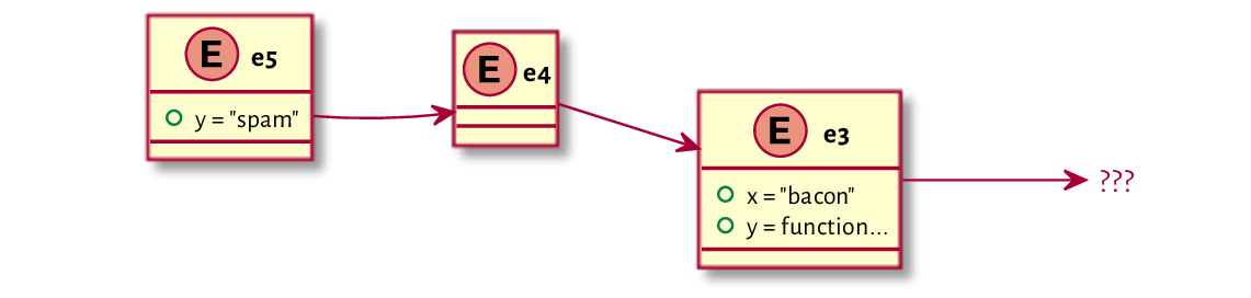
Figure 16.1 Example environments and their enclosures (original setting).

Let’s evaluate the name y in the foregoing environments:

expr_y <- quote(y)
eval(expr_y, envir=e3)
## function() "a function `y` in e3"
eval(expr_y, envir=e5)
## [1] "spam"

No surprises, yet. However, evaluating it in e4, which does not define y, yields:

eval(expr_y, envir=e4)
## function() "a function `y` in e3"

It returned y from e4’s enclosure, e3. Let’s play about with the enclosures of e5 and e4 so that we obtain the setting depicted in Figure 16.2:

parent.env(e5) <- e3
parent.env(e4) <- e5

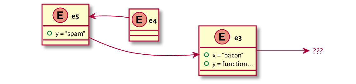
Figure 16.2 Example environments and their enclosures (after the change made).

Evaluating y again in the same e4 nourishes a very different result:

eval(expr_y, envir=e4)
## [1] "spam"

Important

Names referred to in an expression but missing in the current environment will be sought in their enclosure(s) until successful.

Note

Here are the functions related to searching within and modifying environments that optionally allow for continuing explorations in their enclosures:

• inherits=TRUE by default: exists, get,

• inherits=FALSE by default: assign, * rm (remove).

16.2.4. Looking for functions

Interestingly, if a name is used instead of a function to be called, the object sought is always[9] of the mode function. Consider an expression similar to the above, but this time including the name y playing a different role:

expr_y2 <- quote(y())  # a call to something named `y`
eval(expr_y2, envir=e4)
## [1] "a function `y` in e3"

In other words, what we used here was not:

get("y", envir=e4)
## [1] "spam"

but:

get("y", envir=e4, mode="function")
## function() "a function `y` in e3"

Note

name(), "name"(), and `name`() are synonymous. However, the first expression is acceptable only if name is syntactically valid.

16.2.5. Inspecting the search path

Going back to our expression involving a relational operator:

expr_comp
## x < "eggs"

Why does the following work as expected?

eval(expr_comp, envir=e3)  # "bacon" < "eggs"
## [1] TRUE

Well, we have gathered all the bits to understand it now. Namely, `<` is a function that is looked up like:

get("<", envir=e3, inherits=TRUE, mode="function")
## function (e1, e2)  .Primitive("<")

It is reachable from e3, which means that e3 also has an enclosing environment.

parent.env(e3)
## <environment: R_GlobalEnv>

This is our global namespace, which was the current environment when e3 was created. Still, we did not define `<` there. It means that the global environment also has an enclosure.

We can explore the whole search path by starting at the global environment and following the enclosures recursively.

ecur <- globalenv()  # starting point
repeat {
    cat(paste0(format(ecur), " (", attr(ecur, "name"), ")"))  # pretty-print

    if (exists("<", envir=ecur, inherits=FALSE))  # look for `<`
        cat(strrep(" ", 25), "`<` found here!")
    cat("\n")

    ecur <- parent.env(ecur)  # advance to its enclosure
}
## <environment: R_GlobalEnv> ()
## <environment: 0x55e0d2de9088> (.marekstuff)
## <environment: package:stats> (package:stats)
## <environment: package:graphics> (package:graphics)
## <environment: package:grDevices> (package:grDevices)
## <environment: package:utils> (package:utils)
## <environment: package:datasets> (package:datasets)
## <environment: package:methods> (package:methods)
## <environment: 0x55e0d05477f0> (Autoloads)
## <environment: base> ()                          `<` found here!
## <environment: R_EmptyEnv> ()
## Error in parent.env(ecur): the empty environment has no parent

Underneath the global environment, there is a whole list of attached packages:

1. packages attached by the user (.marekstuff is used internally in the process of evaluating code in this book),

2. default packages (Section 7.3.1.1),

3. (**) Autoloads (for the promises-to-load R packages; compare help("autoload"); it is a technicality we may safely ignore here),

4. the base package, which we can access directly by calling baseenv; it is where most of the fundamental functions from the previous chapters reside,

5. the empty environment (emptyenv), which is the only one followed by nil (the loop would turn out endless otherwise).

It comes at no surprise that the `<` operator has been found in the base package.

Note

On a side note, the reason why this operation failed:

e2 <- as.environment(list(x="spam"))  # to recall
eval(expr_comp, envir=e2)
## Error in x < "eggs": could not find function "<"

is because as.environment sets the enclosing environment to:

parent.env(e2)
## <environment: R_EmptyEnv>

See also list2env which gives greater control over this (cf. its parent argument).

16.2.6. Attaching to and detaching from the search path

In Section 7.3.1, we mentioned that we can access the objects exported by a package without attaching them to the search path by using the pkg::object syntax, which loads the package if necessary. For instance:

tools::toTitleCase("`tools` not attached to the search path")
## [1] "`tools` not Attached to the Search Path"

However:

toTitleCase("nope")
## Error in toTitleCase("nope"): could not find function "toTitleCase"

It did not work because toTitleCase is not reachable from the current environment.

Let’s inspect the current search path:

search()
##  [1] ".GlobalEnv"        ".marekstuff"       "package:stats"
##  [4] "package:graphics"  "package:grDevices" "package:utils"
##  [7] "package:datasets"  "package:methods"   "Autoloads"
## [10] "package:base"

Some might find writing “pkg::” inconvenient. Thus, we can call library to attach the package to the search path immediately below the global environment.

library("tools")

The search path becomes (see Figure 16.3 for an illustration):

search()
##  [1] ".GlobalEnv"        "package:tools"     ".marekstuff"
##  [4] "package:stats"     "package:graphics"  "package:grDevices"
##  [7] "package:utils"     "package:datasets"  "package:methods"
## [10] "Autoloads"         "package:base"

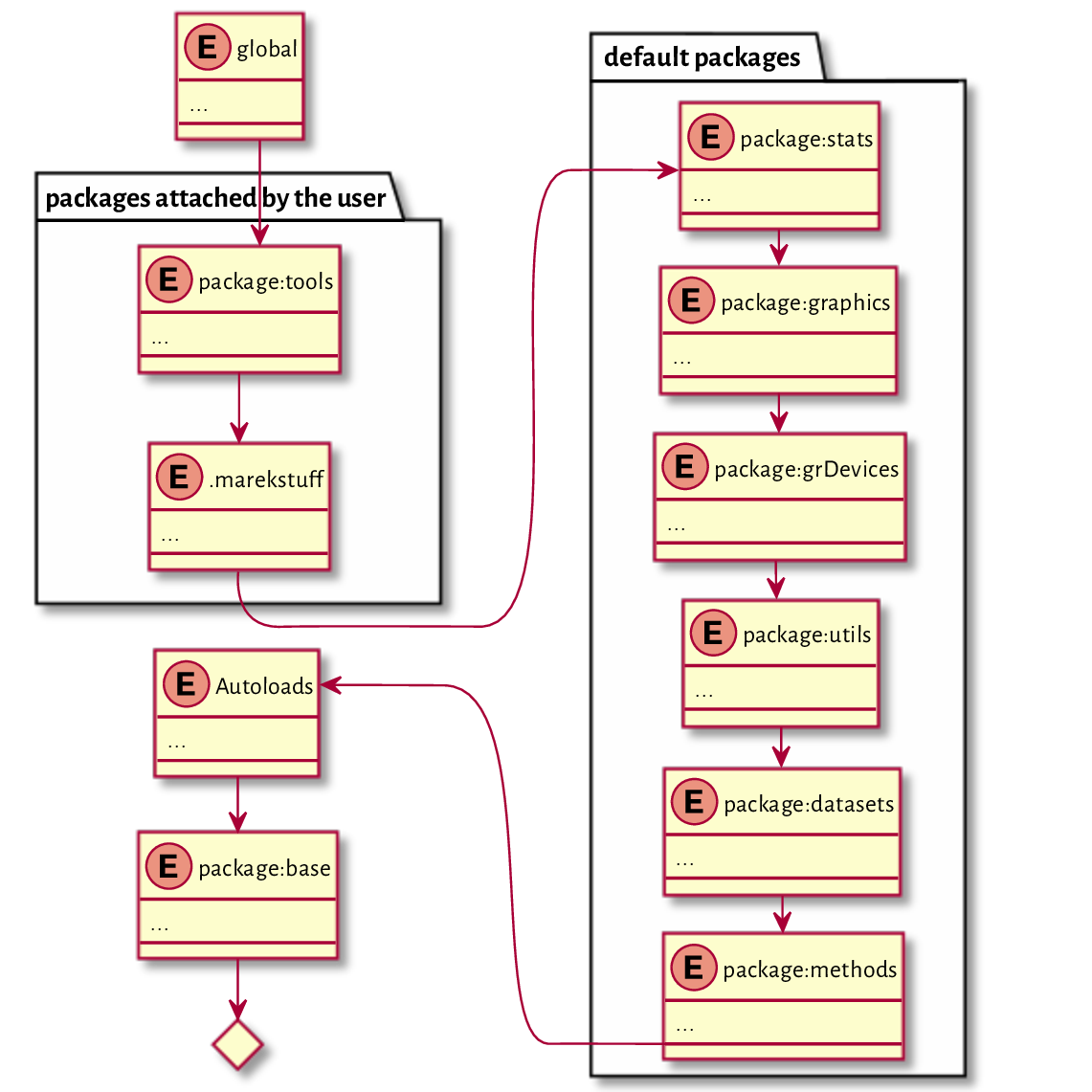
Figure 16.3 The search path after attaching the tools package.

Therefore, what follows, now works as expected:

toTitleCase("Nobody expects the Spanish Inquisition")
## [1] "Nobody Expects the Spanish Inquisition"

We can use detach[10] to remove an item from the search path.

head(search())  # before detach
## [1] ".GlobalEnv"        "package:tools"     ".marekstuff"
## [4] "package:stats"     "package:graphics"  "package:grDevices"
detach("package:tools")
head(search())  # not there anymore
## [1] ".GlobalEnv"        ".marekstuff"       "package:stats"
## [4] "package:graphics"  "package:grDevices" "package:utils"

Note

We can also plug arbitrary environments[11] and named lists into the search path. Recalling that data frames are built on the latter (Section 12.1.6), some users rely on this technique save a few keystrokes.

attach(iris)
head(search(), 3)
## [1] ".GlobalEnv"  "iris"        ".marekstuff"

The iris list was converted to an environment, and the necessary enclosures were set accordingly:

str(parent.env(globalenv()))
## <environment: 0x55e0d20fea08>
##  - attr(*, "name")= chr "iris"
str(parent.env(parent.env(globalenv())))
## <environment: 0x55e0d2de9088>
##  - attr(*, "name")= chr ".marekstuff"

We can now write:

head(Petal.Width/Sepal.Width)  # iris[["Petal.Width"]]/iris[["Sepal.Width"]]
## [1] 0.057143 0.066667 0.062500 0.064516 0.055556 0.102564

Overall, attaching data frames is discouraged, especially outside the interactive mode. Let’s not be too lazy.

detach(iris)  # such a relief

16.2.7. Masking (shadowing) objects from down under

An assignment via `<-` creates a binding in the current environment. Therefore, even if the name to bind exists somewhere on the search path, it will not be modified. Instead, a new name will be created.

eval(quote("spam" < "eggs"))
## [1] FALSE

Here, we rely on `<` from the base environment. Withal, we can create an object of the same name in the current (global) context:

`<` <- function(e1, e2)
{
    warning("This is not the base `<`, mate.")
    NA
}

Now we have two different functions of the same name. When we evaluate an expression within the current environment or any of its descendants, the new name shadows the base one:

"spam" < "eggs"  # evaluate in the global environment
## Warning in "spam" < "eggs": This is not the base `<`, mate.
## [1] NA
eval(quote("spam" < "eggs"), envir=e5)  # its enclosure's enclosure is global
## Warning in "spam" < "eggs": This is not the base `<`, mate.
## [1] NA

But we can still call the original function directly:

base::`<`("spam", "eggs")
## [1] FALSE

It is also reachable from within the current environment’s ancestors:

eval(quote("spam" < "eggs"), envir=parent.env(globalenv()))
## [1] FALSE

Before proceeding any further, we should clean up after ourselves. Otherwise, we will be asking for trouble.

rm("<")  # removes `<` from the global environment

An attached package may introduce some object names that are also available elsewhere. For instance:

library("stringx")
## Attaching package: 'stringx'
## The following objects are masked from 'package:base': casefold, chartr,
##     endsWith, gregexec, gregexpr, grep, grepl, gsub, ISOdate, ISOdatetime,
##     nchar, nzchar, paste, paste0, regexec, regexpr, sprintf, startsWith,
##     strftime, strptime, strrep, strsplit, strtrim, strwrap, sub, substr,
##     substr<-, substring, substring<-, Sys.time, tolower, toupper, trimws,
##     xtfrm, xtfrm.default

Therefore, in the current context, we have what follows:

toupper("Groß")  # stringx::toupper
## [1] "GROSS"
base::toupper("Groß")
## [1] "GROß"

Sometimes[12], we can use assign(..., inherits=TRUE) or its synonym, `<<-`, to modify the existing binding. A new binding is only created if necessary.

Note

Let’s attach the iris data frame (named list) to the search path again:

attach(iris)
Sepal.Length[1] <- 0

We did not modify the original iris nor its converted-to-an-environment copy that we can find in the search path. Instead, a new vector named Sepal.Length was created in the current environment:

exists("Sepal.Length", envir=globalenv(), inherits=FALSE)  # it is in global
## [1] TRUE
Sepal.Length[1]  # global
## [1] 0

We can verify the preceding statement as follows:

rm("Sepal.Length")  # removes the one in the global environment
Sepal.Length[1]  # `iris` from the search path
## [1] 5.1
iris[["Sepal.Length"]][1]  # the original `iris`
## [1] 5.1

However, we can write:

Sepal.Length[1] <<- 0  # uses assign(..., inherits=TRUE)

We changed the state of the environment on the search path.

exists("Sepal.Length", envir=globalenv(), inherits=FALSE)  # not in global
## [1] FALSE
Sepal.Length[1]  # `iris` from the search path
## [1] 0

Yet, the original iris object is left untouched. There is no mechanism in place that would synchronise the original data frame and its independent copy on the search path.

iris[["Sepal.Length"]][1]  # the original `iris`
## [1] 5.1

It is best to avoid attach to avoid confusion.

16.3. Closures

So far, we have only covered the rules of evaluating standalone R expressions. In this section, we look at what happens inside the invoked functions.

16.3.1. Local environment

When we call a function, a new temporary environment is created. It is where all argument values[13] and local variables are emplaced. This environment is the current one while the function is being evaluated. After the call, it ceases to exist, and we return to the previous environment from the call stack.

Consider the following function:

test <- function(x)
{
    print(ls())  # list object names in the current environment
    y <- x^2  # creates a new variable
    print(sys.frame(sys.nframe()))  # get the ID of the current environment
    str(as.list(sys.frame(sys.nframe())))  # display its contents
}

First call:

test(2)
## [1] "x"
## <environment: 0x55e0d2d725b0>
## List of 2
##  $ y: num 4
##  $ x: num 2

Second call:

test(3)
## [1] "x"
## <environment: 0x55e0d34df1d8>
## List of 2
##  $ y: num 9
##  $ x: num 3

Each time, the current environment is different. This is why we do not see the variable y at the start of the second call. It is a brilliantly simple implementation of the storage for local variables.

16.3.2. Lexical scope and function closures

We were able to access the print function (amongst others) in the preceding example. This should make us wonder what the enclosing environment of that local environment is.

print_enclosure <- function()
    print(parent.env(sys.frame(sys.nframe())))

print_enclosure()
## <environment: R_GlobalEnv>

It is the global environment. Let’s invoke the same function from another one:

call_print_enclosure <- function()
    print_enclosure()

call_print_enclosure()
## <environment: R_GlobalEnv>

It is the global environment again. If R used the so-called dynamic scoping, we would see the local environment of the function that invoked the one above. If this was true, we would have access to the caller’s local variables from within the callee. But this is not the case.

Important

Objects of the type closure, i.e., user-defined[14] functions, consist of three components:

• a list of formal arguments (compare formals in Section 15.4.1);

• an expression (see body in Section 15.4.1);

• a reference to the associated environment where the function might store data for further use (see environment).

By default, the associated environment is set to the current environment where the function was created.

A local environment created during a function’s call has this associated environment as its closure.

Due to this, we say that R has lexical (static) scope.

Thence, in the foregoing example, we have:

environment(print_enclosure)  # print the associated environment
## <environment: R_GlobalEnv>

Example 16.7

Consider a function that prints out x defined outside of its scope:

test <- function() print(x)

Now:

x <- "x in global"
test()
## [1] "x in global"

It printed out x from the user workspace as it is precisely the environment associated with the function. However, setting the associated environment to another one that also happens to define x will give a different result:

environment(test) <- e3  # defined some time ago
test()
## [1] "bacon"

Example 16.8

Consider the following:

test <- function()
{
    cat(sprintf("test: current env: %s\n", format(sys.frame(sys.nframe()))))

    subtest <- function()
    {
        e <- sys.frame(sys.nframe())
        cat(sprintf("subtest: enclosing env: %s\n", format(parent.env(e))))
        cat(sprintf("x = %s\n", x))
    }

    x <- "spam"
    subtest()
    environment(subtest) <- globalenv()
    subtest()
}

x <- "bacon"
test()
## test: current env: <environment: 0x55e0d27dc2c0>
## subtest: enclosing env: <environment: 0x55e0d27dc2c0>
## x = spam
## subtest: enclosing env: <environment: R_GlobalEnv>
## x = bacon

Here is what happened.

1. A call to test creates a local function subtest, whose associated environment is set to the local frame of the current call. It is precisely the current environment where subtest was created (because R has lexical scope).

2. The above explains why subtest can access the local variable x inside its maker.

3. Then we change the environment associated with subtest to the global one.

4. In the next call to subtest, unsurprisingly, we gain access to x in the user workspace.

Note

In lexical (static) scoping, which variables a function refers to can be deduced by reading the function’s body only and not how it is called in other contexts. This is the theory. Nevertheless, the fact that we can freely modify the associated environment anywhere can complicate the program analysis greatly.

If we find the rules of lexical scoping complicated, we should refrain from referring to objects outside of the current scope (“global” or “non-local” variables”) except for the functions defined as top-level ones or imported from external packages. It is what we have been doing most of the time anyway.

16.3.3. Application: Function factories

As closures are functions with associated environments, and the role of environments is to store information, we can consider closures = functions + data. We have already seen that in Section 9.4.3, where we mentioned approxfun. To recall:

x <- seq(0, 1, length.out=11)
f1 <- approxfun(x, x^2)
print(f1)
## function (v)
## .approxfun(x, y, v, method, yleft, yright, f, na.rm)
## <environment: 0x55e0d2f5da50>

The variables x, y, etc., that f1’s source code refers to, are stored in its associated environment:

ls(envir=environment(f1))
## [1] "f"      "method" "na.rm"  "x"      "y"      "yleft"  "yright"

Important

Routines that return functions whose non-local variables are memorised in their associated environments are referred to as function factories.

Example 16.9

Consider a function factory:

gen_power <- function(p)
    function(x) x^p  # p references a non-local variable

A call to gen_power creates a local environment that defines one variable, p, where the argument’s value is stored. Then, we create a function whose associated environment (remember that R uses lexical scoping) is that local one. It is where the reference to the non-local p in its body will be resolved. This new function is returned by gen_power to the caller. Normally, the local environment would be destroyed, but it is still used after the call. Thus, it will not be garbage-collected.

Example calls:

(square <- gen_power(2))
## function(x) x^p
## <environment: 0x55e0d200f7f0>
(cube <- gen_power(3))
## function(x) x^p
## <environment: 0x55e0d2081c70>
square(2)
## [1] 4
cube(2)
## [1] 8

The underlying environment can, of course, be modified:

assign("p", 7, envir=environment(cube))
cube(2)  # so much for the cube
## [1] 128

Example 16.10

Negate is another example of a function factory. The function it returns stores f passed as an argument.

notall <- Negate(all)
notall(c(TRUE, TRUE, FALSE))
## [1] TRUE

Study its source code:

print(Negate)
## function (f)
## {
##     f <- match.fun(f)
##     function(...) !f(...)
## }
## <environment: namespace:base>

Example 16.11

In [37], the following example is given:

account <- function(total)
    list(
        balance  = function() total,
        deposit  = function(amount) total <<- total+amount,
        withdraw = function(amount) total <<- total-amount
    )

Robert <- account(1000)
Ross <- account(500)
Robert$deposit(100)
Ross$withdraw(150)
Robert$balance()
## [1] 1100
Ross$balance()
## [1] 350

We can now fully understand why this code does what it does. The return list consists of three functions whose enclosing environment is the same. account somewhat resembles the definition of a class with three methods and one data field. No wonder why reference classes (Section 16.1.5) were introduced at some point: they are based on the same concept.

Exercise 16.12

Write a function factory named gen_counter which implements a simple counter that is increased by one on each call thereto.

gen_counter <- function() ...to.do...
c1 <- gen_counter()
c2 <- gen_counter()
c(c1(), c1(), c2(), c1(), c2())
## [1] 1 2 1 3 2

Moreover, compose a function that resets a given counter to zero.

reset_counter <- function(counter_fun) ...to.do...
reset_counter(c1)
c1()
## [1] 1

16.3.4. Accessing the calling environment

We know that the environment associated with a function is not necessarily the same as the environment from which the function was called, sometimes confusingly referred to as the parent frame.

R maintains a whole frame stack. The global environment is assigned the number 0. Each call to a function increases the stack by one frame, whereas returning from a call decreases the counter. To get the current frame number, we call sys.nframe. This is why sys.frame(sys.nframe()) returns the current environment.

We can fetch the calling environment by referring to parent.frame() or sys.frame(sys.parent()), amongst others[15]. Thanks to parent.frame, we may evaluate arbitrary expressions in (on behalf of) the calling environment. Normally, we should never be doing that. However, a few functions rely on this feature, hence our avid interest in this possibility.

16.3.5. Package namespaces (*)

An R package pkg defines two environments:

• namespace:pkg is where all objects are defined (functions, vectors, etc.); it is the enclosing environment of all closures in the package;

• package:pkg contains selected[16] objects from namespace:pkg that can be accessed by the user; it can be attached to the search path.

As an illustration, we will use the example package discussed in Section 7.3.1.2.

library("rpackagedemo")  # https://github.com/gagolews/rpackagedemo/
## Loading required package: tools

Here is its DESCRIPTION file:

Package: rpackagedemo
Type: Package
Title: Just a Demo R Package
Version: 1.0.2
Date: 1970-01-01
Author: Anonymous Llama
Maintainer: Unnamed Kangaroo <roo@inthebush.au>
Description: Provides a function named bamboo(), just give it a shot.
License: GPL (>= 2)
Imports: stringx
Depends: tools

The Import and Depends fields specify which packages (apart from base) ours depends on. As we can see above, all items in the latter list are attached to the search path on a call to library.

The NAMESPACE file specifies the names imported from other packages and those that are expected to be visible to the user:

importFrom(stringx, sprintf)
importFrom(tools, toTitleCase)
S3method(print, koala)
S3method(print, kangaroo, .a_hidden_method_to_print_a_roo)
export(bamboo)

Thus, our package exports one object, a function named bamboo (we will discuss the S3 methods in the next section). It is included in the package:rpackagedemo environment attached to the search path:

ls(envir=as.environment("package:rpackagedemo")) # ls("package:rpackagedemo")
## [1] "bamboo"

Let’s give it a shot:

bamboo("spanish inquisition")  # rpackagedemo::bamboo
## G'day, Spanish Inquisition!

We did not expect this at all, nor that its source code looks like:

print(bamboo)
## function (x = "world")
## cat(prepare_message(toTitleCase(x)))
## <environment: namespace:rpackagedemo>

We see a call to toTitleCase (most likely from tools, and this is indeed the case). Also, prepare_message is invoked but it is not listed in the package’s imports (see the NAMESPACE file). We definitely cannot access it directly:

prepare_message
## Error in eval(expr, envir, enclos): object 'prepare_message' not found

It is the package’s internal function, which is included in the namespace:rpackagedemo environment.

(e <- environment(rpackagedemo::bamboo))  # or getNamespace("rpackagedemo")
## <environment: namespace:rpackagedemo>
ls(envir=e)
## [1] "bamboo"          "prepare_message" "print.koala"

We can fetch it via the `:::` operator:

print(rpackagedemo:::prepare_message)
## function (x)
## sprintf("G'day, %s!\n", x)
## <environment: namespace:rpackagedemo>

All functions defined in a package have the corresponding namespace as their associated environment. As a consequence, bamboo can refer to prepare_message directly.

It will be educative to inspect the enclosure of namespace:rpackagedemo:

(e <- parent.env(e))
## <environment: 0x55e0d2d48380>
## attr(,"name")
## [1] "imports:rpackagedemo"
ls(envir=e)
## [1] "sprintf"     "toTitleCase"

It is the environment carrying the bindings to all the imported objects. This is why our package can also refer to stringx::sprintf and tools::toTitleCase. Its enclosure is the namespace of the base package (not to be confused with package:base):

(e <- parent.env(e))
## <environment: namespace:base>

The next enclosure is, interestingly, the global environment:

(e <- parent.env(e))
## <environment: R_GlobalEnv>

Then, of course, the whole search path follows; see Figure 16.4 for an illustration.

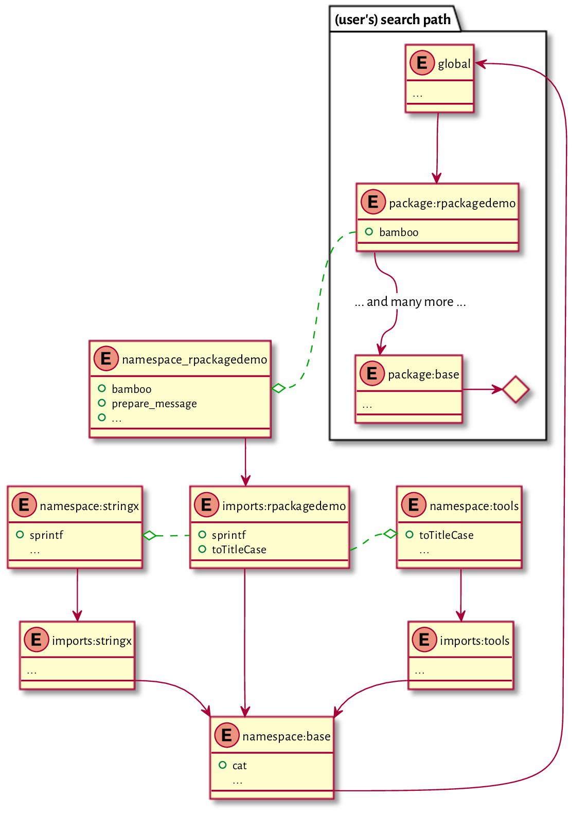
Figure 16.4 A search path for an example package. Dashed lines represent environments associated with closures, whereas solid lines denote enclosing environments. References to objects within each package are resolved inside their respective namespaces.

Note

(**) All environments related to packages are locked, which means that we cannot change any bindings inside their frames; compare help("lockEnvironment"). In the extremely rare event of our needing to patch an existing function within an already loaded package, we can call unlockBinding followed by assign to change its definition.

new_message <- function (x) sprintf("Nobody expects %s!\n", x)
e <- getNamespace("rpackagedemo")
environment(new_message) <- e  # set enclosing environment (very important!)
unlockBinding("prepare_message", e)
assign("prepare_message", new_message, e)
rm("new_message")
bamboo("the spanish inquisition")
## Nobody expects The Spanish Inquisition!

R is indeed a quite hackable language (except in the cases where it is not).

Exercise 16.13

(**) A function or a package might register certain functions (hooks) to be called on various events, e.g., attaching a package to the search patch; see help("setHook") and help(".onAttach").

1. Inspect the source code of plot.new and notice a reference to a hook named "before.plot.new". Try setting such a hook yourself (e.g., one that changes some of the graphics parameters discussed in Section 13.2) and see what happens on each call to a plotting function.

2. Define the .onLoad, .onAttach, .onUnload, and .onDetach functions in your own R package and take note of when they are invoked.

Exercise 16.14

(**) For the purpose of this book, we have registered a custom "before.plot.new" hook that sets our favourite graphics parameters that we listed in Section 13.2.3. Moreover, to obtain a white grid on a grey background, e.g., in Figure 13.13, we modified plot.window slightly. Apply similar hacks to the graphics package so that its outputs suit your taste better.

16.3.6. S3 method lookup by UseMethod (*)

Inspecting the NAMESPACE file in rpackagedemo, we see that the package defines two print methods for objects of the classes koala and kangaroo. As the package is still attached to the search path, we can access these methods via a call to the corresponding generic:

print(structure("Tiny Teddy", class="koala"))
## This is a cute koala, Tiny Teddy
print(structure("Moike", class="kangaroo"))
## This is a very naughty kangaroo, Moike

The package does not make the definitions of these S3 methods available to the user, at least not directly. It is not the first time when we have experienced such an obscuration. In the first case, the method is simply hidden in the package namespace because it was not marked for exportation in the NAMESPACE file. However, it is still available under the expected name:

rpackagedemo:::print.koala
## function (x, ...)
## cat(sprintf("This is a cute koala, %s\n", x))
## <environment: namespace:rpackagedemo>

In the second case, the method appears under a very different identifier:

rpackagedemo:::.a_hidden_method_to_print_a_roo
## function (x, ...)
## cat(sprintf("This is a very naughty kangaroo, %s\n", x))
## <environment: namespace:rpackagedemo>

Since the base UseMethod is still able to find them, we suspect that there must be a global register of all S3 methods. And this is indeed the case. We can use getS3method to get access to what is available via UseMethod:

getS3method("print", "kangaroo")
## function (x, ...)
## cat(sprintf("This is a very naughty kangaroo, %s\n", x))
## <environment: namespace:rpackagedemo>

Important

Overall, the search for methods is performed in two places:

1. in the environment where the generic is called (the current environment); this is why defining print.kangaroo in the current scope will use this method instead of the one from the package:

   print.kangaroo <- function(x, ...) cat("Nobody expects", x, "\n")
   print(structure("the Spanish Inquisition", class="kangaroo"))
   ## Nobody expects the Spanish Inquisition
   

2. in the internal S3 methods table (registration database).

See help("UseMethod") for more details. Also, recall that in Section 10.2.3, we said that UseMethod is not the only way to perform method dispatching. There are also internal generics and group generic functions.

Exercise 16.15

(*) Study the source code of getS3method. Note the reference to the base::`.__S3MethodsTable__.` object which is for R’s internal use (we ought not to tinker with it directly). Moreover, study the .S3method function with which we can define new S3 methods not necessarily following the generic.classname convention.

16.4. Exercises

Exercise 16.16

Asking too many questions is not very charismatic, but challenge yourself by finding the answer to the following.

• What is the role of a frame in an environment?

• What is the role of an enclosing environment? How to read it or set it?

• What is the difference between a named list and an environment?

• What functions and operators work on named lists but cannot be applied on environments?

• What do we mean by saying that environments are not passed by value to R functions?

• What do we mean by saying that objects are sometimes copied on demand?

• What happens if a name listed in an expression to be evaluated is not found in the current environment?

• How and what kind of objects can we attach to the search path?

• What happens if we have two identical object names on the search path?

• What do we mean by saying that package namespaces are locked when loaded?

• What is the current environment when we evaluate an expression “on the console”?

• What is the difference between `<-` and `<<-`?

• Do packages have their own search paths?

• What is a function closure?

• What is the difference between the dynamic and the lexical scope?

• When evaluating a function, how is the enclosure of the current (local) environment determined? Is it the same as the calling environment? How to get it/them programmatically?

• How and why function factories work?

• (*) What is the difference between the package:pkg and namespace:pkg environments?

• How do we fetch the definition of an S3 method that does not seem to be available directly via the standard accessor generic.classname?

• (*) base::print.data.frame calls base::format.data.frame (directly). Will the introduction of print.data.frame in the current environment affect how data frames are printed?

• (*) On the other hand, base::format.data.frame calls the generic base::format on all the input data frame’s columns. Will the overloading of the particular methods affect how data frames are printed?

Exercise 16.17

Calling:

pkg <- available.packages()
pkg[, "Package"]  # a list of the names of available packages
pkg[, "Depends"]  # dependencies

gives the list of available packages and their dependencies. Convert the dependency lists to a list of character vectors (preferably using regular expressions; see Section 6.2.4).

Then, generate a list of reverse dependencies: what packages depend on each given package.

Use an object of the type environment (a hash table) to map the package names to numeric IDs (indexes). It will significantly speed up the whole process (compare it to a named list-based implementation).

Exercise 16.18

According to [69], compare also Section 9.3.6, a call to:

add(x, f(x)) <<- v

translates to:

`*tmp*` <- get(x, envir=parent.env(), inherits=TRUE)
x <<- `add<-`(`*tmp*`, f(x), v)  # note: not f(`*tmp*`)
rm(`*tmp*`)

Given:

`add<-` <- function(x, where=TRUE, value)
{
    x[where] <- x[where] + value
    x  # the modified object that will replace the original one
}

y <- 1:5
f <- function() { y <- -(1:5); add(y, y==-3) <<- 1000; y }

explain why we get the following results:

f()
## [1] -1 -2 -3 -4 -5
print(y)
## [1]    1    2 1003    4    5

---

[1]

Not to be confused with a data frame, i.e., an object (list) of the S3 class data.frame; see Chapter 12.

[2]

Some also call it a parent environment, but we will not. We will try to follow the nomenclature established in Section 3.2 of [1]. Note that there is a bit of a mess in the R documentation regarding how enclosing environments are referred to.

[3]

Accessing elements by position (numeric index) in lists takes \(O(1)\) time. The worst-case runtime for the element lookup by name is linear with respect to the container size (when the item is not found). Also, inserting new elements at the end takes amortised \(O(1)\) time.

[4]

Delayed (on demand); see below.

[5]

We do not count all the tricks we can do at the C language level (Chapter 14). In R, the distinction between pass-by-value and pass-by-reference is slightly more complicated because of the lazy evaluation of arguments (the call-by-need strategy; Chapter 17). We have made an idealisation for didactic purposes.

[6]

Some call them R5, but we will not.

[7]

That is why everyone serious about R programming should add the Structure and Interpretation of Computer Programs [1] to their reading list. Also, R is not the only known marriage between statistics and Lisp-like languages; see also LISP-STAT [54].

[8]

For now, let’s take for granted that `<-` is accessible from the current context and denotes the assignment.

[9]

This is why we can write “c <- c(1, 2)” and then still be able to call c to create another vector.

[10]

Which does not unload the package from memory, though; see unload (possibly combined with library.dynam.unload).

[11]

Or we should rather say, environment frames. When an environment is attached to the search path, it is duplicated so that the changes made to the original environment are not reflected in the copy. Then, its previous enclosure is discarded. After all, we want a series of recursive calls to parent.env to form the whole search path.

[12]

We normally cannot modify package namespaces. As we will mention in Section 16.3.5, they are automatically locked.

[13]

Function arguments are initially unevaluated; see Chapter 17.

[14]

There are two other types of functions: a special is an internal function that does not necessarily evaluate its arguments (e.g., switch, if, or quote; compare also Chapter 17), whereas a builtin always evaluates its actual parameters, e.g., sum.

[15]

In help("sys.parent"), we read that the parent frame number, as returned by sys.parent(), is not necessarily equal to sys.nframe()-1. It is certainly true if we are at the top (global) level.

[16]

Exported using the export or exportPattern directive in the package’s NAMESPACE file; see Section 1 of [65].